

The volatility smile forces us to leave the flatland of constant volatility and model volatility as a dynamic quantity. This article introduces local volatility (LV) models, contrasts them with stochastic volatility (SV), presents Bruno Dupire’s non‑parametric model, discusses practical implementation and visualization, and finally offers a pragmatic parametric alternative: the Constant Elasticity of Variance (CEV) model with calibration guidance and Python code.
1. A New Paradigm: Local vs. Stochastic Volatility
The Black–Scholes–Merton (BSM) framework assumes constant volatility. Real markets display a smile (or skew) of implied volatilities across strikes and maturities, forcing a rethink of volatility modeling.
Two broad model families emerged to explain this gap:
1.1 Local Volatility (LV) Models
Local volatility models treat volatility as a deterministic function of the current asset price St and time t:

By construction, a LV model is calibrated to reproduce exactly the observed European option prices at a single point in time. In other words, LV models are interpolation tools: they answer the question “what deterministic diffusion would produce today’s option surface?”
1.2 Stochastic Volatility (SV) Models
Stochastic volatility models treat volatility as its own stochastic process. A generic SV system can be written as:
$$
dS(t) = \mu S(t)\,dt + v(t)S(t)\,dW_{1}(t) \\
dv(t) = \alpha(S,v,t)\,dt + \eta v(t)\,dW_{2}(t)
$$
where v(t) (variance) follows its own SDE and the Brownian drivers W1 and W2 can be correlated. SV models naturally capture empirically observed dynamics such as volatility clustering and more realistic time‑evolution of the smile.
1.3 The Practitioner’s Trade‑off
- LV models: easy to calibrate (fit today’s smile exactly), but their forward dynamics can be unrealistic. Often the smile flattens too quickly over time, which may misprice long‑dated or path‑dependent payoffs.
- SV models: more realistic dynamics, better for risk simulations and hedging, but harder and costlier to calibrate and not guaranteed to match today’s smile exactly.
Choosing between these families is philosophical: do you need a model that interpolates today’s liquid vanilla market accurately (LV) or one that plausibly generates future price dynamics for risk management (SV)?
2. Dupire’s Equation: Deriving Local Volatility from Prices
Bruno Dupire showed (1994) that for any arbitrage‑free surface of European option prices C(K,T), there exists a unique local volatility function sigma(K,T) under risk‑neutral dynamics that is consistent with those prices. Dupire’s formula links local variance directly to partial derivatives of call option prices:
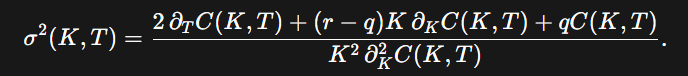
Here r is the risk‑free rate and q the continuous dividend yield. The numerator captures time decay (Theta) and drift adjustments; the denominator is the strike convexity (dual gamma). The formula is a reverse‑engineering device: given the full surface of vanilla prices, it reveals the local volatility that must have generated them.
Intuition
Local variance is proportional to time decay and inversely proportional to convexity in strike. Where option prices decay faster in time but have strong convexity with strike, local variance increases.
3. Building the Volatility Surface in Practice
Dupire’s theory is elegant but numerically treacherous. Implementing it requires care through several steps:
3.1 Steps
- Data assembly. Collect quoted option prices C(Ti,Kj) across a grid of maturities and strikes.
- Surface smoothing / interpolation. Market quotes are discrete and noisy. Fit a smooth, arbitrage‑free surface (bivariate splines, kernel regressions, or other smoothers). This is the most important practical step.
- Numerical differentiation. Compute \(\partial_T C\), \(\partial_K C\), and \(\partial^2_{K} C\) using finite differences on the smoothed surface.
- Apply Dupire. Plug derivatives into Dupire’s formula to obtain sigma(K,T) across the grid.
3.2 Numerical fragility
Calculating a second derivative amplifies noise. Small jitter in the smoothed price surface can make \(\partial^2_{K} C\) tiny or even non‑positive, producing infinite or imaginary local vols. Thus the smoothing/interpolation step is not optional — it is the single biggest determinant of success.
4. Visualizing the Landscape
A 3D plot of the local volatility surface is the most intuitive representation: time to maturity on one axis, strike or moneyness on the second, and local volatility on the vertical axis. A slice at fixed maturity recovers the original smile.
import matplotlib.pyplot as plt
from matplotlib import cm
import numpy as np

def plot_local_vol_surface(maturities, strikes, local_vol_grid):
    """
    Plots the 3D local volatility surface.

    Args:
        maturities (np.array): 1D array of maturities.
        strikes (np.array): 1D array of strikes.
        local_vol_grid (np.array): 2D array of local volatilities,
                                  with shape (len(strikes), len(maturities)).
    """
    # Create meshgrid for plotting
    T, K = np.meshgrid(maturities, strikes)

    fig = plt.figure(figsize=(12, 8))
    ax = fig.add_subplot(111, projection='3d')

    # Plot the surface
    surface = ax.plot_surface(T, K, local_vol_grid, cmap=cm.viridis,
                              linewidth=0, antialiased=True, alpha=0.9)

    # Customize the plot
    ax.set_title('Local Volatility Surface')
    ax.set_xlabel('Time to Maturity (Years)')
    ax.set_ylabel('Strike Price')
    ax.set_zlabel('Local Volatility')

    # Add a color bar which maps values to colors.
    fig.colorbar(surface, shrink=0.5, aspect=5)

    # Set viewing angle
    ax.view_init(elev=30., azim=-60)

    plt.show()

# Example usage with dummy data:
# maturities = np.linspace(0.1, 2.0, 20)
# strikes = np.linspace(80, 120, 25)
# # In a real application, local_vol_grid would be the output of the Dupire calculation
# local_vol_grid = np.random.rand(len(strikes), len(maturities)) * 0.2 + 0.15
# plot_local_vol_surface(maturities, strikes, local_vol_grid)
5. A Pragmatic Solution — The Constant Elasticity of Variance (CEV) Model
Dupire’s non‑parametric approach is powerful but delicate. Practitioners often sacrifice flexibility for robustness via parametric LV models. The CEV model is a classic choice.
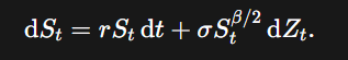
Under risk‑neutral dynamics the CEV SDE is:
Key parameters:
- σ : volatility scale.
- β (elasticity): typically 0≤β<2
The instantaneous variance is

so when β<2 the variance increases as the price falls — capturing the leverage effect and generating the downward skew seen in equities. When β=2 the model reduces to geometric Brownian motion (BSM).
5.2 Pricing: non‑central chi‑square
For β<2 the European call price admits a closed form involving non‑central chi‑square CDFs (see Hsu et al.). The result can be written:

where the intermediate quantities are

This closed form stems from mapping the process to a squared Bessel process: transition densities are non‑central chi‑square.
5.3 Python implementation (pricer)
from scipy.stats import ncx2

def cev_price(S, K, T, r, sigma, beta, option_type='call'):
    """
    Calculates the price of a European option using the CEV model.
    This implementation follows Hsu et al. (2008).

    Args:
        S (float): Current price of the underlying asset.
        K (float): Strike price of the option.
        T (float): Time to expiration in years.
        r (float): Risk-free interest rate (annualized).
        sigma (float): Volatility scaling parameter.
        beta (float): Elasticity parameter (0 <= beta < 2).
        option_type (str): 'call' or 'put'.

    Returns:
        float: The CEV price of the option.
    """
    if T <= 0:
        if option_type == 'call':
            return max(0.0, S - K)
        elif option_type == 'put':
            return max(0.0, K - S)
        else:
            raise ValueError("Invalid option type.")

    # Prevent division by zero or log(0) issues
    if sigma <= 0 or S <= 0:
        return np.nan

    # The case beta = 2 corresponds to the BSM model (lognormal)
    # A separate handler would be needed for that case. We focus on beta < 2.
    if beta >= 2:
        raise ValueError("Beta must be less than 2 for this formula.")

    # Calculate intermediate parameters
    v = 2 / (2 - beta)
    kappa = (2 * r) / (sigma**2 * (2 - beta) * (np.exp(r * (2 - beta) * T) - 1))

    x = kappa * (S**(2 - beta)) * np.exp(r * (2 - beta) * T)
    y = kappa * (K**(2 - beta))

    # Degrees of freedom and non-centrality parameters for the ncx2 cdf
    df_x = 2 + v
    nc_x = 2 * x

    df_y = v
    nc_y = 2 * y

    # Calculate the non-central chi-square CDF values
    cdf1 = ncx2.cdf(2 * y, df_x, nc_x)
    cdf2 = ncx2.cdf(2 * x, df_y, nc_y)

    # Calculate call price
    call_price = S * (1 - cdf1) - K * np.exp(-r * T) * cdf2

    if option_type == 'call':
        return call_price
    elif option_type == 'put':
        # Use put-call parity to find the put price
        put_price = call_price - S + K * np.exp(-r * T)
        return put_price
    else:
        raise ValueError("Invalid option type.")

# Example Usage with assumed parameters from source material
# S0 = 142.7 # Assuming this is the spot price for the IBM example
# K = 140
# T = 64 / 365 # Dec 17, 2021 from Oct 14, 2021
# r = 0.05 # Assumed risk-free rate
# sigma_guess = 0.35
# beta_guess = 1.25
# price = cev_price(S0, K, T, r, sigma_guess, beta_guess, 'call')
# print(f"CEV Call Price (uncalibrated): {price:.4f}")
5.4 Calibration
Calibration of the CEV model means finding the parameter pair (σ,β) that best explains the observed market option prices or implied volatilities. Because the CEV model has only two parameters, the optimization is tractable and stable compared to richer models.
Step 1: Define the Objective
The most common calibration objective is the sum of squared errors (SSE) between model‑produced option prices and observed market prices:

where wi are optional weights (e.g., proportional to option liquidity). Alternatively, we can match implied volatilities directly:

The second approach gives a more uniform fit across strikes, since raw prices differ by orders of magnitude between deep ITM and OTM options.
Step 2: Choose Constraints
- σ>0 for positivity of volatility.
- 0≤β<2. When β=2 the model collapses to BSM; values below 2 capture skew.
Step 3: Select an Optimization Algorithm
Practical methods include:
- Grid search (for small problems, to visualize the error landscape).
- Nonlinear least squares (e.g.,
scipy.optimize.least_squares). - Global optimizers like differential evolution if local minima are suspected.
A two‑step approach often works best: run a global optimizer coarsely, then refine with local least‑squares.
Step 4: Evaluate the Fit
- Plot model vs. market option prices across strikes.
- Compare implied volatilities from CEV vs. observed smile.
- Compute metrics such as mean squared error (MSE) or mean absolute percentage error (MAPE).
from scipy.optimize import minimize

def cev_calibration_objective(params, market_prices, S, K, T, r, option_type='call'):
    """
    Objective function for CEV model calibration.
    Calculates the sum of squared errors between model and market prices.

    Args:
        params (list or tuple): A list containing [sigma, beta].
        market_prices (np.array): Array of observed market prices.
        S, K, T, r: Market data inputs for the pricer. K is an array.

    Returns:
        float: The sum of squared errors.
    """
    sigma, beta = params

    # Handle cases where parameters might go out of bounds during optimization
    if sigma <= 0 or beta < 0 or beta >= 2:
        return 1e9 # Return a large number to penalize invalid parameter sets

    model_prices = np.array([cev_price(S, k, T, r, sigma, beta, option_type) for k in K])

    # Ensure no NaN values in model_prices, which can happen with extreme params
    if np.isnan(model_prices).any():
        return 1e9

    error = np.sum((model_prices - market_prices)**2)
    return error

# --- Calibration Execution ---
# Assume we have: S0, T, r, and two arrays: strikes_market, prices_market
# 1. Initial guess for parameters
# initial_guess = [0.3, 1.0]

# 2. Bounds for the parameters [ (sigma_min, sigma_max), (beta_min, beta_max) ]
# bounds = [(1e-3, 2.0), (0.0, 1.99)]

# 3. Run the optimization
# 'L-BFGS-B' is a good choice as it handles bounds.
# result = minimize(
#     fun=cev_calibration_objective,
#     x0=initial_guess,
#     args=(prices_market, S0, strikes_market, T, r),
#     method='L-BFGS-B',
#     bounds=bounds,
#     options={'ftol': 1e-8} # Set a tolerance for convergence
# )

# 4. Extract the optimal parameters
# if result.success:
#     calibrated_sigma, calibrated_beta = result.x
#     print(f"Calibration successful!")
#     print(f"Calibrated Sigma: {calibrated_sigma:.4f}")
#     print(f"Calibrated Beta: {calibrated_beta:.4f}")
# else:
#     print(f"Calibration failed: {result.message}")
Interpretation of Results
- Low β: stronger skew — implied volatilities fall more sharply with strike.
- High β: closer to BSM — flatter smile.
- Sigma: scales overall volatility level.
The calibrated pair (σ∗,β∗) must be re‑estimated periodically, as option smiles evolve with market conditions.
Conclusion
Local volatility models provide a rigorous way to reproduce today’s vanilla option surface exactly. Dupire’s formula is a powerful theoretical result, but direct implementation is numerically sensitive and requires careful smoothing. Parametric alternatives like the CEV model trade perfect flexibility for stability and interpretability. With only two parameters, CEV captures the crucial skew through a simple elasticity parameter and is straightforward to calibrate in practice.
The modeling journey does not end here. For richer dynamics, practitioners turn to stochastic volatility models or hybrid Stochastic‑Local‑Volatility (SLV) setups that combine the calibration fidelity of LV with the realistic dynamics of SV. Volatility modeling remains an active dialogue between market observation and theoretical innovation.