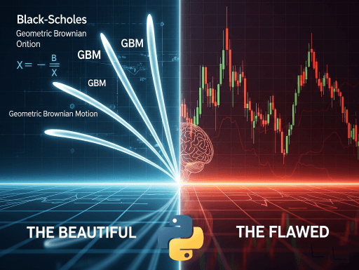
A Quant’s Guide to the Beautiful, Flawed Formulas That Run Wall Street

Hey there! Ever looked at the stock market and thought it moves like a hyperactive squirrel that’s had too much espresso? Well, you’re not wrong. Welcome to the wild, wacky, and wonderful world of quantitative finance.

Our mission, should you choose to accept it, is to learn how to speak the language of financial randomness. We’ll build some of the most powerful models in finance from the ground up, peek under the hood to see how they work, and most importantly figure out their limits. Think of this as learning to cook a gourmet meal, but also learning that sometimes you’re just going to burn the toast. And that’s okay!

Taming the Chaos — The Language of Randomness

First thing’s first: finance is all about uncertainty. Sure, some things are predictable, like a government bond payment (thanks, Uncle Sam!). But the price of Apple stock tomorrow? Or the exchange rate in the next 60 seconds? That’s all up to chance. To model this, we need to learn the language of stochastic processes.

That sounds fancy, but it’s just a “choose-your-own-adventure” story for numbers. It’s a process that evolves over time, guided by a bit of randomness. Unlike a boring old deterministic process where Start A always leads to End B, a stochastic process says that from Start A, you could end up at B, C, D, or Z, each with a different probability.

Here’s your starter vocabulary:

• Random Variable: A variable whose value is a surprise party waiting to happen. Think of a stock’s daily return, you don’t know what it’ll be until it happens!
• State Space: The complete menu of all possible values your random variable can choose from. For a stock price, this is any number from zero to infinity.
• Time Index: When we decide to peek at our random variable. It can be discrete (like checking the closing price every day) or continuous (watching the price tick by tick).
• Path: A single, complete story of how our random variable played out over time. The S&P 500’s journey over the next year is one path out of a bajillion possibilities.

Finance’s “Short-Term Memory”: The Markov Property

Now, let’s talk about a super important concept in finance models: the Markov Property.

Imagine a goldfish. Its world is new every few seconds. It doesn’t remember how it got to its corner of the tank; it only knows where it is right now. A process with the Markov property is exactly like that goldfish, its future only depends on its present state and not the past path it took to get there. This is often called the “memoryless” property.

In finance, this assumes a stock’s future price depends only on its current price. All the dramatic twists and turns from yesterday or last year? The model says, “Nope, don’t care, already baked into today’s price.” This is basically the weak-form efficient market hypothesis (EMH) in a snazzy mathematical disguise. It says you can’t beat the market just by looking at old price charts.

The name comes from botanist Robert Brown, who saw pollen grains doing a chaotic jig in water. He realized they were being knocked around by zillions of tiny, invisible water molecules. This “drunken sailor’s walk” is the perfect metaphor for the random, unpredictable dance of asset prices.

A Wiener process (W_t) has two key features:

1. Normally Distributed Increments: The change over a tiny bit of time (∆t) is random and follows a bell curve (a Normal distribution). The variance of this change is equal to the time step ∆t.
2. Independent Increments: The sailor’s step from yesterday to today has zero influence on his step from today to tomorrow. This connects directly back to that “memoryless” Markov property we just talked about.

import numpy as np
import matplotlib.pyplot as plt
def simulate_wiener_process(T, N):
    """
    Simulates a 1D standard Wiener process (Brownian motion).
    Args:
        T (float): Total time horizon.
        N (int): Number of time steps.
    Returns:
        tuple: A tuple containing the time axis and the simulated Wiener path.
    """
    # Time step size
    dt = T / N      
    # Generate random increments from a normal distribution
    # The increments are dW = epsilon * sqrt(dt)
    # We generate N standard normal random numbers (epsilon) and scale them
    increments = np.random.normal(0, np.sqrt(dt), N)        
    # Create the time axis
    t = np.linspace(0, T, N + 1)        
    # Cumulatively sum the increments to get the path
    # We start the path at 0
    W = np.zeros(N + 1)
    W[1:] = np.cumsum(increments)        
    return t, W
# --- Simulation Parameters ---
T = 1.0  # Time horizon of 1 year
N = 500  # Number of steps
# --- Run Simulation ---
time_axis, wiener_path = simulate_wiener_process(T, N)
# --- Plotting ---
plt.figure(figsize=(10, 6))
plt.plot(time_axis, wiener_path)
plt.title('Simulated Path of a Standard Wiener Process')
plt.xlabel('Time (t)')
plt.ylabel('Value (W_t)')
plt.grid(True)
plt.show()

Here’s its secret recipe, written as a stochastic differential equation (SDE):

dSₜ ​= Sₜ​ ( μdt + σdWₜ ​)

Let’s break that down:

• dSₜ: The teeny-tiny change in the stock price (S) right now.
• μSₜdt (The Drift): This is the predictable part. It’s the underlying trend of the stock, based on its expected return, μ. Think of it as the gentle wind at the sailor’s back.
• σSₜdWₜ (The Shock): This is the random part. It’s the unpredictable wobble, where dWₜ is our drunken sailor’s step. This wobble is scaled by the stock’s volatility, σ.

The absolute genius of GBM is that it guarantees the stock price never goes below zero. Because we’re modeling proportional changes, the price follows a log-normal distribution. Unlike a normal distribution (a symmetric bell curve), a log-normal distribution is skewed and can’t be negative. Problem solved!

import numpy as np
import matplotlib.pyplot as plt
def simulate_gbm(S0, mu, sigma, T, N, num_paths):
    """
    Simulates multiple paths of Geometric Brownian Motion.
    Args:
        S0 (float): Initial stock price.
        mu (float): Expected return (drift).
        sigma (float): Volatility.
        T (float): Total time horizon.
        N (int): Number of time steps.
        num_paths (int): Number of paths to simulate.
    """
    dt = T / N
    t = np.linspace(0, T, N + 1)
    
    # Generate random increments for all paths at once
    # Z has shape (N, num_paths)
    Z = np.random.normal(0, 1, (N, num_paths))
    
    # Calculate the log returns
    log_returns = (mu - 0.5 * sigma**2) * dt + sigma * np.sqrt(dt) * Z
    # This is discretized term for our SDE, after applying Ito's lemma
    # Not sure? Just ask in comments, i will explain
    
    # Prepend zeros for the initial log price
    log_returns = np.vstack([np.zeros(num_paths), log_returns])
    
    # Calculate the cumulative log returns
    cumulative_log_returns = np.cumsum(log_returns, axis=0)
    
    # Exponentiate to get the price paths
    price_paths = S0 * np.exp(cumulative_log_returns)
    
    return t, price_paths
# --- Simulation Parameters ---
S0 = 100.0       # Initial stock price
mu = 0.05        # Expected annual return of 5%
sigma = 0.20     # Annual volatility of 20%
T = 1.0          # Time horizon of 1 year
N = 252          # Number of trading days in a year
num_paths = 10   # Number of simulated paths
# --- Run Simulation ---
time_axis, price_paths = simulate_gbm(S0, mu, sigma, T, N, num_paths)
# --- Plotting ---
plt.figure(figsize=(12, 7))
plt.plot(time_axis, price_paths)
plt.title(f'{num_paths} Simulated Geometric Brownian Motion Paths')
plt.xlabel('Time (Years)')
plt.ylabel('Stock Price ($)')
plt.grid(True)
plt.show()

See? All the paths start at $100, but they forge their own random destinies, and none of them crash through the floor to become negative.

You can’t use regular calculus here. The path of Brownian motion is so jagged and twitchy that it’s technically not differentiable anywhere. We need a new tool: Itô’s Lemma, the chain rule for random stuff.

The magic of Itô’s Lemma comes down to one weird, non-intuitive rule: (dW_t)² =dt. In normal calculus, any tiny thing squared becomes so small it just vanishes. Not here! In the stochastic world, the squared random change doesn’t disappear, it equals a tiny step in time. This little fact is what makes stochastic calculus different and is the key to everything that follows.

The Black-Scholes-Merton Model

Armed with Itô’s Lemma, Fischer Black, Robert Merton, and Myron Scholes built the most famous equation in all of finance, which won them a Nobel Prize. The Black-Scholes-Merton (BSM) model gives us a theoretical price for a European option.

The absolute genius of their idea was hedging. They realized you could create a portfolio with one option and a specific amount of the underlying stock that, for a split second, is completely risk-free. How? By choosing the amount of stock (the option’s Delta, Δ) so that the random up-and-down wobbles from the stock and the option perfectly cancel each other out.

And what do we know about risk-free assets? In a world with no free lunch (no arbitrage), they must earn exactly the risk-free interest rate, r.

By setting the change in this risk-free portfolio equal to the risk-free rate, they derived the BSM partial differential equation:

The most magical thing happened: the stock’s expected return, μ, completely vanished from the equation! The option’s price doesn’t depend on whether you think the stock will go to the moon. It only depends on the current price (S), volatility (sigma), time (T), strike price (K), and the risk-free rate (r).

This leads to a powerful trick called risk-neutral valuation. We can price the option by pretending we live in a world where all assets grow at the risk-free rate, r. It’s not real, but the hedging argument guarantees it gives the right price for our world.

Solving that PDE gives us the famous Black-Scholes formulas.

For a European Call Option:

For a European Put Option:

Where:

• d_1, d_2

• N(.) is the cumulative distribution function for a standard normal variable (a fancy way of saying “the probability of getting a result less than this value”).

import numpy as np
from scipy.stats import norm
def black_scholes_pricer(S, K, T, r, sigma, option_type='call'):
    """
    Calculates the price of a European option using the Black-Scholes-Merton model.
    """
    d1 = (np.log(S / K) + (r + 0.5 * sigma**2) * T) / (sigma * np.sqrt(T))
    d2 = d1 - sigma * np.sqrt(T)
    
    if option_type == 'call':
        N_d1 = norm.cdf(d1)
        N_d2 = norm.cdf(d2)
        price = (S * N_d1) - (K * np.exp(-r * T) * N_d2)
    elif option_type == 'put':
        N_minus_d1 = norm.cdf(-d1)
        N_minus_d2 = norm.cdf(-d2)
        price = (K * np.exp(-r * T) * N_minus_d2) - (S * N_minus_d1)
    else:
        raise ValueError("Invalid option type. Choose 'call' or 'put'.")
    
    return price
# --- Input Parameters ---
S = 100.0      # Current stock price
K = 105.0      # Strike price
T = 1.0        # 1 year to expiration
r = 0.05       # 5% risk-free rate
sigma = 0.20   # 20% volatility
# --- Calculate Option Prices ---
call_price = black_scholes_pricer(S, K, T, r, sigma, option_type='call')
put_price = black_scholes_pricer(S, K, T, r, sigma, option_type='put')
print(f"The theoretical price of the European Call option is: ${call_price:.2f}")
print(f"The theoretical price of the European Put option is: ${put_price:.2f}")

Another Reality Check! The “Beautiful Lie” of BSM The BSM model is elegant, but it’s built on a foundation of assumptions that are, let’s be honest, pretty sketchy in the real world.

Constant Volatility? LOL. The model assumes volatility (σ) is constant. This is its most famously violated assumption. In reality, if you look at options with different strike prices, they will give you different implied volatilities, forming a pattern called the “volatility smile” or “skew”. The BSM model can’t explain this at all.

Normal Returns? Nope, “Fat Tails”. The model assumes returns follow a nice, tame normal distribution. Real market returns have “fat tails,” meaning crazy, extreme price swings happen way more often than the model predicts. BSM systematically underestimates the risk of a market crash.

Your Risk Dashboard: The Greeks

The BSM model also gives us the “Greeks,” which are vital signs for your option’s risk. They tell you how sensitive your option’s price is to different factors.

• Delta: How much the option price changes when the stock moves by $1.
• Gamma: How much your Delta changes when the stock moves by $1. It’s the acceleration of your option’s value.
• Vega: Sensitivity to changes in volatility. (Higher volatility is good for option holders!).
• Theta: Sensitivity to the passage of time. It’s the “time decay” that slowly eats away at your option’s value as it nears expiration.

When Formulas Fail, We Brute Force It: Monte Carlo

The BSM formula is sleek and fast, but it only works for simple, “vanilla” European options. What if you have a complex “exotic” option, like an Asian option whose payoff depends on the average price over its life? There’s no clean formula for that.

Enter the Monte Carlo method. It’s the ultimate “brute force” technique. The idea is simple:

1. Simulate: Use the risk-neutral GBM formula to simulate thousands upon thousands of possible future stock prices.
2. Calculate Payoff: For each simulated price, calculate what the option’s payoff would be.
3. Average: Find the average of all those payoffs.
4. Discount: Discount that average back to today’s value using the risk-free rate.

Voilà! That’s your option price. It’s a direct application of the idea that an option’s price is just the expected value of its future payoffs.

def monte_carlo_pricer(S, K, T, r, sigma, num_simulations, option_type='call'):
    """
    Prices a European option using Monte Carlo simulation.
    """
    # Generate random numbers from a standard normal distribution
    Z = np.random.normal(0, 1, num_simulations)
    
    # Simulate the stock price at expiration T
    ST = S * np.exp((r - 0.5 * sigma**2) * T + sigma * np.sqrt(T) * Z)
    
    # Calculate the option payoff for each simulated path
    if option_type == 'call':
        payoffs = np.maximum(ST - K, 0)
    elif option_type == 'put':
        payoffs = np.maximum(K - ST, 0)
    else:
        raise ValueError("Invalid option type. Choose 'call' or 'put'.")
    
    # Discount the average payoff to get the option price
    price = np.mean(payoffs) * np.exp(-r * T)
    
    return price
# --- Input Parameters (same as BSM example) ---
S = 100.0
K = 105.0
T = 1.0
r = 0.05
sigma = 0.20
num_simulations = 100000
# --- Calculate Option Prices ---
mc_call_price = monte_carlo_pricer(S, K, T, r, sigma, num_simulations, 'call')
bsm_call_price = black_scholes_pricer(S, K, T, r, sigma, 'call') # Using previous function
print(f"Monte Carlo Call Price: ${mc_call_price:.4f}")
print(f"Black-Scholes Call Price: ${bsm_call_price:.4f}")

Final Reality Check: Patience, Young Grasshopper The law of large numbers promises that as you increase the number of simulations, the Monte Carlo price will get closer and closer to the true price (like the BSM price for a vanilla option). But this takes time! If you only run 1,000 simulations, your answer could be way off just due to statistical noise. Getting a highly accurate price can require millions of paths. So if your result looks “unsuccessful,” don’t blame the model just yet, you might just need to let your computer run for a bit longer!

The Takeaway

And there you have it! We went from pure chaos to building models that won a Nobel Prize. The key thing to remember is that these models are powerful tools, not crystal balls. They are all “useful fictions” built on simplifying assumptions.

Thinking like a true quant means understanding not just the formulas, but also their limitations and the trade-offs involved. It’s about knowing when a model is the perfect tool for the job, and when its assumptions are going to crash and burn in the face of messy, complicated reality. Now go forth and model responsibly!