Machine Learning for Quants (Part 4)

Introduction

Welcome to the part 4 of the Machine Learning for Quants series. In Parts 1–3, we focused on Time Series data (predicting stock movements). Now, we shift to Cross-Sectional Data; analyzing a snapshot of many different entities at a single point in time.

We will tackle one of the most critical tasks in banking and quantitative risk: Credit Default Prediction. Banks use these models to determine the “Probability of Default” (PD) for loan applicants. This determines interest rates and capital requirements.

This case study brings together everything we have learned: Logistic Regression, Scaling, and Evaluation Metrics and introduces the challenge of Imbalanced Data and Non-Linear Feature Engineering.

Learning Objectives

By the end of this tutorial, you will be able to:

• Differentiate between Time Series (Market) and Cross-Sectional (Risk) modeling workflows.
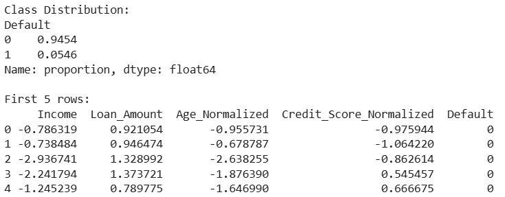
• Handle Imbalanced Data, where “Defaults” are rare events (1% vs 99%).
• Apply Polynomial Features to capture non-linear relationships (e.g., how Age affects risk).
• Compare Models using ROC Curves to select the best risk engine.

Prerequisites

• Completion of Part 3: Familiarity with Logistic Regression and ROC Curves.
• Libraries: scikit-learn, pandas, numpy, matplotlib, seaborn.

Core Concepts

1. Cross-Sectional vs. Time Series

1. Time Series (Parts 1-3): Order matters. We used shuffle=False because today depends on yesterday.
2. Cross-Sectional (Part 4): Order does not matter. Customer A’s default risk is independent of Customer B’s. We must shuffle the data to ensure our Training and Test sets are representative.

2. The Imbalanced Class Problem

In credit risk, most people pay back their loans. A dataset might have 95% “Good” payers (Class 0) and only 5% “Defaulters” (Class 1).

• The Trap: A model that predicts “No Default” for everyone achieves 95% Accuracy but is useless to the bank.
• The Fix: We rely heavily on ROC/AUC and Confusion Matrices, not Accuracy. We may also use class_weight=’balanced’ to tell the model to pay more attention to the rare defaults.

3. Non-Linearity in Risk

Risk is rarely linear.

• Linear Assumption: “Older is always safer.”
• Reality: Very young people (no history) are risky. Very old people (fixed income) might also be risky. Middle-aged people might be safest.
• To capture this “U-shape,” we introduce Polynomial Features ($Age^2$), allowing the Linear/Logistic model to fit curves.

The Hands-On Practice

Step 1: Generating the Dataset

Since we cannot share proprietary bank data, we will generate a realistic synthetic dataset representing 10,000 loan applicants.

import numpy as np

import pandas as pd

import matplotlib.pyplot as plt

import seaborn as sns

from sklearn.datasets import make_classification

 

# 1. Generate Synthetic Data

# We create 10,000 samples, 4 features.

# weights=[0.95, 0.05] creates an imbalance (5% defaults)

X, y = make_classification(n_samples=10000, n_features=4, n_informative=3,

n_redundant=0, n_clusters_per_class=1,

weights=[0.95, 0.05], random_state=42)

 

# 2. Convert to DataFrame for readability

columns = [‘Income’, ‘Loan_Amount’, ‘Age_Normalized’, ‘Credit_Score_Normalized’]

df = pd.DataFrame(X, columns=columns)

df[‘Default’] = y

 

# 3. Inspect the Imbalance

print(“Class Distribution:”)

print(df[‘Default’].value_counts(normalize=True))

 

print(“nFirst 5 rows:”)

print(df.head())

 

Step 2: Preprocessing (Split & Scale)

Because this is cross-sectional data, we randomly shuffle the split.

from sklearn.model_selection import train_test_split

from sklearn.preprocessing import StandardScaler

 

# Define Features and Target

X = df.drop(‘Default’, axis=1)

y = df[‘Default’]

 

# 1. Random Split (Shuffle=True is default, but good to be explicit)

X_train, X_test, y_train, y_test = train_test_split(X, y, test_size=0.2, random_state=42, shuffle=True)

 

# 2. Scale Features

scaler = StandardScaler()

X_train_scaled = scaler.fit_transform(X_train)

X_test_scaled = scaler.transform(X_test)

 

print(f“Training set: {X_train.shape}”)

print(f“Test set: {X_test.shape}”)

 

Step 3: Baseline Logistic Regression

We train a standard model to establish a baseline.

from sklearn.linear_model import LogisticRegression

from sklearn.metrics import classification_report, roc_auc_score, confusion_matrix

 

# Initialize Model (Standard)

model_base = LogisticRegression()

model_base.fit(X_train_scaled, y_train)

 

# Predict

y_pred = model_base.predict(X_test_scaled)

y_prob = model_base.predict_proba(X_test_scaled)[:, 1]

 

# Evaluate

print(“Baseline Classification Report:”)

print(classification_report(y_test, y_pred))

 

print(f“Baseline AUC Score: {roc_auc_score(y_test, y_prob):.4f}”)

 

# Visualizing the Imbalance in Confusion Matrix

cm = confusion_matrix(y_test, y_pred)

sns.heatmap(cm, annot=True, fmt=‘d’, cmap=‘Reds’)

plt.title(“Confusion Matrix (Baseline)”)

plt.xlabel(“Predicted”)

plt.ylabel(“Actual”)

plt.show()

 

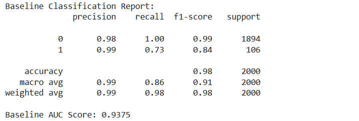
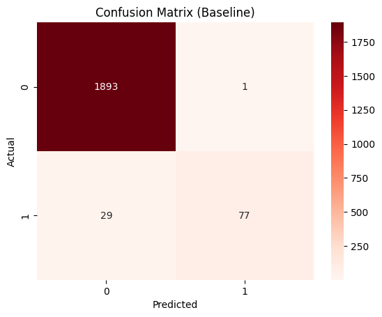
Observation: You notice the model predicts very few defaults (Low Recall for Class 1). It plays it safe.

Step 4: Adding Complexity (Polynomial Features)

Let’s try to capture non-linear risk factors (like the Age curve mentioned earlier) to improve performance.

from sklearn.preprocessing import PolynomialFeatures

 

# 1. Create Polynomial Features (Degree 2)

# This creates interaction terms: Income^2, Income*Age, Age^2, etc.

poly = PolynomialFeatures(degree=2, include_bias=False)

 

X_train_poly = poly.fit_transform(X_train_scaled)

X_test_poly = poly.transform(X_test_scaled)

 

print(f“New Feature Count: {X_train_poly.shape[1]} (Original was 4)”)

 

# 2. Train New Model on Complex Data

# We use ‘class_weight=balanced’ to help the model pay attention to rare defaults

model_poly = LogisticRegression(class_weight=‘balanced’, solver=‘liblinear’)

model_poly.fit(X_train_poly, y_train)

 

# Predict

y_prob_poly = model_poly.predict_proba(X_test_poly)[:, 1]

 

print(f“Polynomial Model AUC Score: {roc_auc_score(y_test, y_prob_poly):.4f}”)

 

Step 5: Comparing Performance (ROC Curves)

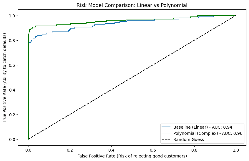
Visualizing which model is better at separating good borrowers from risky ones.

from sklearn.metrics import roc_curve

 

# Calculate ROC for Baseline

fpr_base, tpr_base, _ = roc_curve(y_test, y_prob)

 

# Calculate ROC for Polynomial

fpr_poly, tpr_poly, _ = roc_curve(y_test, y_prob_poly)

 

# Plot

plt.figure(figsize=(10, 6))

plt.plot(fpr_base, tpr_base, label=f‘Baseline (Linear) – AUC: {roc_auc_score(y_test, y_prob):.2f}’)

plt.plot(fpr_poly, tpr_poly, label=f‘Polynomial (Complex) – AUC: {roc_auc_score(y_test, y_prob_poly):.2f}’, color=‘green’)

plt.plot([0, 1], [0, 1], ‘k–‘, label=‘Random Guess’)

 

plt.xlabel(‘False Positive Rate (Risk of rejecting good customers)’)

plt.ylabel(‘True Positive Rate (Ability to catch defaults)’)

plt.title(‘Risk Model Comparison: Linear vs Polynomial’)

plt.legend()

plt.show()

 

Check Your Work

• Imbalance Check: In Step 1, verify that Default 1 is roughly 5% of the data.
• Feature Expansion: In Step 4, if you started with 4 features and used Degree 2, you should end up with roughly 14 features ($N + N + text{interactions}$).
• Curve Check: The Polynomial ROC curve (Green) should generally be higher (closer to the top left) than the Baseline curve (Blue).

Challenge: Business Thresholds

Banks don’t just want an AUC; they want a decision.

1. Assume the bank accepts a loan if the Probability of Default < 20%.
2. Write a script that filters the test set for y_prob_poly < 0.20.
3. Calculate the Default Rate of this “Accepted Portfolio.” It should be significantly lower than the global average of 5%.

Conclusion

In this tutorial: We successfully built a Credit Scoring engine. We handled class imbalance and proved that adding non-linear complexity (Polynomials) significantly improves our ability to detect risky borrowers compared to a simple linear model.

You now possess the foundational toolkit of a Quantitative Machine Learning practitioner: Data Engineering, Supervised Learning, Regularization, and Rigorous Evaluation.

Troubleshooting / FAQ

Q: My Polynomial Model is taking a long time to train.

A: Polynomial features expand the dataset rapidly. If you use degree=3 or higher, the number of features explodes. For most financial tasks, degree=2 is sufficient.

Q: Why use solver=’liblinear’?

A: Standard Logistic Regression solvers can sometimes struggle to converge on complex, high-dimensional datasets. liblinear is often more robust for smaller-to-medium datasets.

Q: The Polynomial model has a worse Accuracy but better AUC. Why?

A: This is the class_weight=’balanced’ effect. The model is willing to make more False Positives (rejecting some good customers) to ensure it catches the Defaults. This lowers pure “Accuracy” but improves the “Safety” of the bank (AUC), which is the true goal.