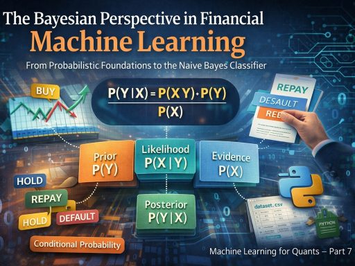
From Probabilistic Foundations to the Naive Bayes Classifier (ML for Quants: Part 7)

Introduction to Supervised Learning in Finance

In last module of this curriculum, we explored unsupervised machine learning, where the goal was to find hidden structures within unlabeled data. We now transition again into Supervised Machine Learning. In this paradigm, we deal with labeled data: we have input variables (predictors/features) and a known target variable. Our objective is to build a model that maps the inputs to the target with high accuracy.

This article focuses on one of the most fundamental probabilistic approaches to classification: Bayesian Statistics. Specifically, we will examine how Bayes’ Theorem can be applied to predict binary financial outcomes such as whether a stock should be a “Buy” or “Hold,” or whether a loan applicant will “Default” or “Repay.” We will traverse the theoretical derivation of the theorem, the assumptions behind the “Naive” Bayes classifier, and finally, a robust implementation using Python.

Section 1: The Bayesian Framework

To understand Bayesian statistics, we must first ground ourselves in the concept of conditional probability. In classical frequentist statistics, we often view probability as the long-run frequency of events. However, the Bayesian view interprets probability as a measure of belief or certainty about an event, which is updated as more evidence becomes available.

1.1 Collective Exhaustive Events

In binary classification problems, we often deal with a collectively exhaustive set of events. This means the set of all possible outcomes covers 100% of the possibilities.

If we define an event A (e.g., a company defaults), and its complement \(\overline{A}\) (the company does not default), then:

1.2 Conditional Probability and Derivation

Bayesian analysis relies heavily on conditional probability; the probability of an event occurring given that another event has already occurred.

Let:

• Y: The target variable (Class), e.g., Default (1) or No Default (0).
• X: The predictor variable (Feature), e.g., “Employed for < 3 years”.

Since both equations equal $P(Y cap X)$, we can set them equal to each other:

1.3 The Components of Bayes’ Theorem

Section 2: The “Naive” Assumption

While the independence assumption is rarely 100% true in financial data (e.g., a company’s “Debt” and “Interest Expense” are correlated), the Naive Bayes classifier often performs surprisingly well in practice because the direction of the correlation often points to the correct class, even if the exact probability estimate is slightly biased.

Section 4: Practical Implementation in Python

We will now implement a Gaussian Naive Bayes classifier using Python and scikit-learn. We will simulate a scenario where we predict whether a stock provides a positive return (Class 1) or negative return (Class 0) based on two factors.

4.1 Step 1: Library Import and Data Generation

First, we import the necessary libraries. We will use sklearn.naive_bayes.GaussianNB for the model and generate synthetic data to demonstrate the mechanics clearly.

import numpy as np
import pandas as pd
import matplotlib.pyplot as plt
from sklearn.naive_bayes import GaussianNB
from sklearn.model_selection import train_test_split
from sklearn.metrics import confusion_matrix, accuracy_score, classification_report
 
# Generating synthetic financial data
# Feature 1: Momentum (Continuous)
# Feature 2: Value Score (Continuous)
np.random.seed(42)
n_samples = 1000
 
# Generating "Good" stocks (Class 1)
good_momentum = np.random.normal(0.5, 1.0, 500)
good_value = np.random.normal(0.5, 1.0, 500)
labels_good = np.ones(500)
 
# Generating "Bad" stocks (Class 0)
bad_momentum = np.random.normal(-0.5, 1.0, 500)
bad_value = np.random.normal(-0.5, 1.0, 500)
labels_bad = np.zeros(500)
 
# Combining data
X = np.column_stack((np.concatenate([good_momentum, bad_momentum]),
                     np.concatenate([good_value, bad_value])))
y = np.concatenate([labels_good, labels_bad])
 
print(f"Data Shape: {X.shape}")

4.2 Step 2: Splitting Data

We must separate our data into training and testing sets to evaluate performance on unseen data.

X_train,X_test,y_train,y_test =train_test_split(X,y,test_size=0.25,random_state=42)

4.3 Step 3: Training the Model

We instantiate the GaussianNB classifier. When we call .fit(), the algorithm calculates the prior probabilities $P(Y)$ and the likelihood parameters ($mu$ and $sigma$) for each feature for each class.

# Initialize the Gaussian Naive Bayes classifier
gnb = GaussianNB()
 
# Train the model
gnb.fit(X_train, y_train)
 
# Output the learned priors (Class probability)
print(f"Class Priors (Bad, Good): {gnb.class_prior_}")
print(f"Feature Means (Bad Stocks): {gnb.theta_[0]}")
print(f"Feature Means (Good Stocks): {gnb.theta_[1]}")

4.4 Step 4: Making Predictions

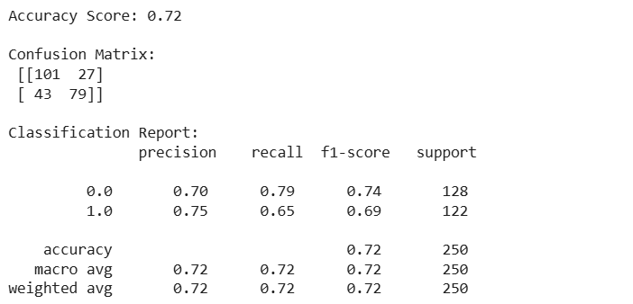
The model calculates the posterior probability for the test set and assigns the class with the highest probability.

# Make predictions
y_pred = gnb.predict(X_test)
 
# Evaluation
print("Accuracy Score:", accuracy_score(y_test, y_pred))
print("\nConfusion Matrix:\n", confusion_matrix(y_test, y_pred))
print("\nClassification Report:\n", classification_report(y_test, y_pred))

Conclusion

The Naive Bayes classifier provides a probabilistic approach to machine learning. By leveraging Bayes’ Theorem, it updates the prior belief of a financial outcome using the evidence provided by new data. Despite the “naive” assumption of feature independence, the Gaussian Naive Bayes model is a powerful baseline tool for continuous financial data, offering speed, interpretability, and solid performance, particularly when data is limited.

In the next part of this series, we will move away from strict probabilistic independence and explore Tree-Based Models, which can capture complex, non-linear interactions between variables.