The Hidden Trap in Your Data: Taming Multicollinearity

In our previous article, we explored the power of linear regression to model relationships between variables. We built both simple and multiple regression models, learning how to interpret their outputs. However, as we add more variables to our models to capture the complexity of the real world, we can stumble into a common but tricky statistical trap: Multicollinearity.

Imagine you’re building a model to predict the price of a house. You include square footage as an independent variable. Then, you also add the number of bedrooms and the number of bathrooms. Intuitively, we know that these three variables are related—larger houses tend to have more bedrooms and bathrooms. When independent variables in a regression model are highly correlated, it can wreak havoc on your results, making them unstable and unreliable. This phenomenon is multicollinearity.

This article will guide you through understanding, detecting, and mitigating multicollinearity. We’ll start with the foundational concepts of covariance and correlation, learn how to visualize these relationships, and then dive deep into the problems caused by multicollinearity. Most importantly, we’ll equip you with practical tools, like the Variance Inflation Factor (VIF), to diagnose and fix this issue in your own models.

Understanding Relationships: Covariance and Correlation

Before we can tackle multicollinearity, we need to understand how to measure the degree to which two variables move together.

Covariance is a measure of the joint variability of two random variables. A positive covariance indicates that the variables tend to move in the same direction, while a negative covariance means they move in opposite directions. However, the magnitude of covariance is hard to interpret because it’s dependent on the units of the variables.

This is where correlation comes in. The correlation coefficient is a standardized version of covariance that is much easier to interpret. It’s a value between -1 and +1 that measures the strength and direction of a linear relationship between two variables.

• Correlation = +1: Perfect positive linear relationship. As one variable increases, the other increases by a proportional amount.
• Correlation = -1: Perfect negative linear relationship. As one variable increases, the other decreases by a proportional amount.
• Correlation = 0: No linear relationship between the variables.

The formula for the sample correlation coefficient (r) between two variables X and Y is:

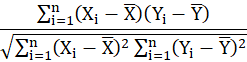
Where X and Y are the sample means of the two variables.

Visualizing Correlation with a Heatmap

Calculating the correlation between every pair of independent variables is the first step in detecting multicollinearity. A correlation matrix is a table showing the correlation coefficients between variables. The best way to visualize this matrix is with a heatmap. The colors in the heatmap give us an immediate sense of which variables are strongly correlated.

import pandas as pd
import seaborn as sns
import matplotlib.pyplot as plt

# Load the dataset
df = pd.read_csv('data.csv')

# Select the variables for our analysis
selected_vars = ['Coke_Q_EX_R', 'Dow_Q_EX_R', 'Pepsi_Q_EX_R', 'GOOG_Q_EX_R', 'BAC_Q_EX_R', 'PFE_Q_EX_R', 'WMT_Q_EX_R', 'HD_Q_EX_R']
df_selected = df[selected_vars]

# Calculate the correlation matrix
corr_matrix = df_selected.corr()

# Plot the heatmap
plt.figure(figsize=(12, 8))
sns.heatmap(corr_matrix, annot=True, cmap='coolwarm', fmt=".2f")
plt.title('Correlation Matrix of Quarterly Excess Returns', fontsize=16)
plt.show()

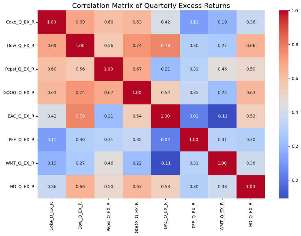
The heatmap shows the correlation coefficient for each pair of variables. Warmer colors (like red) indicate a strong positive correlation, while cooler colors (like blue) indicate a strong negative correlation. For example, we observe a high correlation between Coca-Cola’s returns and Dow’s, Pepsi’s and Google’s. This high correlation is a red flag for multicollinearity if we were to include both in the same model as predictors.

What is Multicollinearity and Why Is It a Problem?

Multicollinearity occurs when independent variables in a regression model are correlated. It doesn’t mean there’s a relationship between an independent variable and the dependent variable (that’s what we want!), but rather between two or more independent variables.

Why is this problematic?

1. Unreliable Coefficients: When two independent variables are highly correlated, the model has a hard time distinguishing their individual effects on the dependent variable. This can lead to wild fluctuations in the coefficient estimates if the model is run on a slightly different sample of data.
2. Inflated Standard Errors: Multicollinearity increases the standard errors of the coefficients. This makes the coefficients seem less statistically significant, and we might wrongly conclude that a variable has no effect on the dependent variable when it actually does.
3. Counterintuitive Signs: The estimated coefficients might have signs that don’t make sense. For example, a variable that should have a positive relationship with the dependent variable might show a negative coefficient.
4. Overfitting: While multicollinearity doesn’t reduce the overall predictive power of the model (R-squared is often high), it can be a symptom of overfitting. The model might perform well on the training data but poorly on new, unseen data.

Detecting Multicollinearity: The Variance Inflation Factor (VIF)

While a correlation matrix is good for spotting pairwise correlations, it can’t detect more complex relationships where one independent variable is a linear combination of multiple other independent variables. For a more robust diagnostic tool, we turn to the Variance Inflation Factor (VIF).

The VIF for an independent variable (Xj) is calculated as:

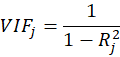
Where R_j² is the R-squared value from a regression of (Xj) on all the other independent variables.

Interpreting VIF:

• VIF = 1: No correlation between the independent variable and the others. This is the ideal scenario.
• 1 < VIF < 5: Moderate correlation. This is generally not a cause for concern.
• VIF > 5: Potentially high correlation. This indicates that the variable may be problematic and warrants further investigation. Some practitioners use a more conservative threshold of 10.

Let’s calculate the VIF for a multiple regression model where we try to predict Coca-Cola’s returns using several other stock returns.

from statsmodels.stats.outliers_influence import variance_inflation_factor
from statsmodels.tools.tools import add_constant

# Define the set of independent variables
X_vif = df[['Dow_Q_EX_R', 'Pepsi_Q_EX_R', 'GOOG_Q_EX_R', 'BAC_Q_EX_R', 'PFE_Q_EX_R']]
X_vif = add_constant(X_vif) # VIF calculation needs an intercept

# Calculate VIF for each variable
vif_data = pd.DataFrame()
vif_data["feature"] = X_vif.columns
vif_data["VIF"] = [variance_inflation_factor(X_vif.values, i) for i in range(X_vif.shape[1])]

print(vif_data)

The output of this code gives us the following table of VIF scores:

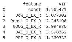
Let’s analyze these results:

• The VIF for the constant (const) is not relevant for our multicollinearity diagnostics.
• Pepsi_Q_EX_R, GOOG_Q_EX_R, and PFE_Q_EX_R all have VIF scores very close to 1. This is excellent! It means they are not correlated with the other independent variables in the model.
• Dow_Q_EX_R (VIF = 5.76) and BAC_Q_EX_R (VIF = 5.73) both have scores greater than 5. This is a clear red flag. It tells us that these two variables are highly correlated with each other and/or with other predictors, which confirms a multicollinearity problem. This makes intuitive sense, as the Dow Jones Industrial Average (a market index) and Bank of America (a major financial institution) are both heavily exposed to the same macroeconomic forces.

How to Handle Multicollinearity

So you’ve found multicollinearity in your model. What now? Here are three common strategies:

• Drop One of the Correlated Variables: This is the simplest approach. Since Dow_Q_EX_R and BAC_Q_EX_R are highly correlated, they are likely capturing similar information about the overall economy. By removing one (for example, BAC_Q_EX_R), we can often solve the multicollinearity issue without losing much explanatory power.
• Combine the Correlated Variables: Instead of dropping a variable, you could combine them. For instance, if you have several correlated variables representing different aspects of firm size, you could create a single “size index” from them. This retains the information from all variables while creating a single, less correlated predictor.
• Use Advanced Methods like Principal Component Analysis (PCA): PCA is a dimensionality reduction technique that transforms your correlated independent variables into a new set of uncorrelated variables called “principal components.” You can then use these components as independent variables in your regression. This is a powerful technique that we will cover in detail in our next article.

Let’s see the effect of dropping a variable. Suppose our VIF calculation showed that Dow_Q_EX_R and BAC_Q_EX_R have high VIFs. We could drop BAC_Q_EX_R and re-run the VIF calculation to see if the problem is resolved.

Conclusion: Building Robust Models

Multicollinearity is a subtle but serious issue that can undermine the reliability of your regression models. It’s a reminder that we can’t just throw variables into a model without thought; we must understand the relationships between our predictors.

In this article, we’ve learned how to use correlation matrices and, more powerfully, the Variance Inflation Factor (VIF) to diagnose multicollinearity. We’ve also discussed practical strategies, like dropping or combining variables, to mitigate it. By carefully checking for and addressing multicollinearity, you can build more robust, stable, and interpretable models.

The journey continues. While we’ve discussed simple fixes, the next article will introduce Principal Component Analysis, a sophisticated and powerful method for dealing with multicollinearity and reducing the dimensionality of your data. Stay tuned!