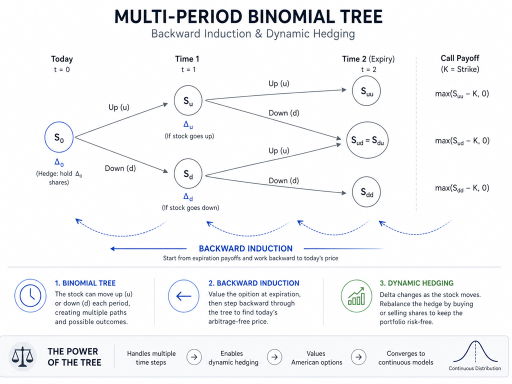
In Chapter 7, we performed a seemingly impossible magic trick. By imagining a highly simplified universe where a stock could only move once per year, we successfully synthetically cloned an option and discovered its exact, mathematically perfect price.

But as you and I both know, the real world doesn’t tick once a year. Stock prices move every month, every day, every minute, and every microsecond. A single-step model is a fantastic teaching tool, but it is useless on a real trading floor.

To bridge the gap between our classroom whiteboard and the high-speed servers of Wall Street, we need to add more time steps. We need to let the tree branch out.

In this chapter, we are going to expand our Binomial Model from a single period to multiple periods. In doing so, we will uncover two massive operational realities of the options market: Dynamic Hedging and the mathematical beauty of Backward Induction.

8.1 Expanding the Temporal Tree: The Two-Period Model

Let’s take our 1-year option from the previous chapter, but instead of allowing the stock to move only once at the end of the year, let’s allow it to move twice; once every six months.

We now have a Two-Period Binomial Tree.

Let’s set up the math. (To keep our focus entirely on the mechanics, we will once again assume the risk-free interest rate (r) is exactly 0%).

1. Current Stock Price (S): $100
2. The “Up” Factor (u): 1.10 (The stock goes up 10% each period).
3. The “Down” Factor (d): 0.90 (The stock goes down 10% each period).

Because the factors are the same, our Risk-Neutral Probability (p) remains the exact same for every single step of the tree:

p=1+0-0.901.10-0.90=0.100.20=0.50

Mapping the Stock Price Paths:

Let’s draw the tree from left to right.

• Today (Node 0): Stock is at $100.
• Month 6 (Node 1): The stock can move UP to $110 or DOWN to $90.
• Month 12 (Node 2: Expiration): From the $110 node, the stock can move UP to $121 (UU) or DOWN to $99 (UD). From the $$90$ node, the stock can move UP to $99 (DU) or DOWN to $81 (DD).

Notice that UD and DU result in the exact same stock price ($99). The tree reconnects with itself. We now have three possible terminal states at expiration: $121, $99, or $81.

8.2 Backward Induction: Solving the Tree

Now that we have the stock prices mapped out, how do we price a Call Option with a $100 Strike?

We cannot simply solve it from left to right. We must start at the very end of the tree (Expiration Day) and work our way backwards to the present day. This computational process is known as Backward Induction.

Step 1: Calculate the Payoffs at Expiration (Month 12)

If we reach Expiration Day, what is our $100 Strike Call worth?

• If stock is $121 (UU Node): Call is worth $21.
• If stock is $99 (UD or DU Node): Call is completely Out-Of-The-Money, worth $0.
• If stock is $81 (DD Node): Call is completely Out-Of-The-Money, worth $0.

Step 2: Step Back to Month 6

Now, we imagine we are standing at Month 6. We have two possible nodes we could be standing on.

1. Imagine we are at the UP node (Stock is $110): We look forward. We see a 50% risk-neutral probability of the option being worth $21, and a 50% probability of it being worth $0.
   1. Expected Value at $110 Node: 0.5×$21+0.5×$0=$10.50.
2. Imagine we are at the DOWN node (Stock is $90): We look forward. We see a 50% probability of $0, and a 50% probability of $0.
   1. Expected Value at $90 Node: $0.00.

Step 3: Step Back to Today (Month 0)

We are back at today. The stock is $100. We look forward to Month 6. We see a 50% probability the option will be worth $10.50, and a 50% probability it will be worth $0.

• Expected Value Today: 0.5×$10.50+0.5×$0=$5.25.

The exact, arbitrage-free price of this option today is $5.25. We solved it by recursively folding the future back into the present.

8.3 The Necessity of Dynamic Hedging

This brings us to the most important operational concept for a derivatives trader. In Chapter 7, we learned that to replicate an option, we needed to buy a specific fractional amount of stock, called Delta (Δ).

Let’s calculate the required Delta at different points in our new two-period tree.

Reminder: Δ=Change in Option Price/Change in Stock Price

Delta Today (Stock is $100):

Looking forward to Month 6, the option price will either be $10.50 or $0. The stock will either be $110 or $90.

• Δ=$10.50-$0/$110-$90
• Δ= $10.50 / $20 = $ 0.525 shares

To replicate the option today, you must buy exactly 0.525 shares.

Fast forward to Month 6. Assume the stock went UP to $110.

Let’s calculate the required Delta now. Looking forward to Month 12, the option will either be $21 or $0. The stock will either be $121 or $99.

• Δ=$21-$0/$121-$99
• Δ= $21 / $22 ≈ 0.95 shares

The Reality of the Trading Floor:

Look closely at what just happened. Today, you only needed 0.525 shares to replicate the option. But six months from now, if the stock goes up, you need 0.95 shares to replicate the option.

Your Replicating Portfolio is not static.

As the stock price moves, the Δ changes. Therefore, to maintain your perfect, risk-free synthetic clone, you must actively enter the market and buy more shares (going from 0.525 to 0.95). If the stock had gone down, you would have had to sell shares.

This constant, mandatory rebalancing of the portfolio is called Dynamic Hedging. This is what market makers do all day long. They don’t place a trade and go to sleep; they are constantly buying and selling the underlying stock as the market ticks to ensure their Δ is perfectly balanced.

8.4 Pricing American Options: The Power of the Tree

So far, we have only priced European options. Why? Because the math for European options is easy; you just look at the expiration day and fold backward.

But what about American Options, which can be exercised at any time?

Mathematical formulas (like Black-Scholes) cannot easily handle the infinite choices of an American option. But the Binomial Tree handles it beautifully.

Because we are using Backward Induction, we are literally calculating the value of the option at every single node in history.

To price an American option, we simply add one logical check at every single node as we move backward: “Is the option worth more ALIVE or DEAD?”

The American Logic Check:

Imagine we are at the Month 6 DOWN node, and we are pricing an American Put Option.

• The “Alive” Value: We calculate the expected value of holding the option into the future (using our p probability). Let’s say the math tells us the continuing value is $4.00.
• The “Dead” Value (Intrinsic Value): We ask, “What if I exercise it right now?” We look at the Strike price and the current Stock price at that node and find the Intrinsic Value. Let’s say the Strike is $100 and the Stock is at $90. The Intrinsic Value is $10.00.

The logical choice is obvious. Why hold an option mathematically worth $4.00 when you can exercise it immediately for $10.00? You would exercise early!

When running the Backward Induction, the computer simply looks at the two numbers (Alive vs. Dead) and chooses the higher number to pass backward to the previous node. This simple logical fork allows the Binomial Tree to perfectly price complex American options, capturing that “Early Exercise Premium” we discussed in Chapter 6.

8.5 From Discrete to Continuous

We started with a 1-step tree. Then we built a 2-step tree.

What if we built a tree with 365 steps (one for every day of the year)? The math is the exact same, we just need a computer (or a Python script) to do the thousands of calculations.

What if we built a tree with 10,000 steps? Or 1 million steps?

As we slice time into infinitesimally smaller discrete steps, the jagged, jagged edges of our binomial tree begin to smooth out. The stock price no longer jumps abruptly; it flows.

If you take a Binomial Tree and expand the number of steps (N) toward infinity, the geometric distribution of the terminal stock prices perfectly converges into a smooth, continuous bell curve (specifically, a log-normal distribution).

By understanding this convergence, you have just intuitively derived the foundation of continuous-time mathematics. You now understand that the terrifying, calculus-heavy Black-Scholes-Merton model is just a Binomial Tree with an infinite number of microscopic steps!

<br>

Chapter Summary

• Multi-Period Expansion: By adding more time steps, the Binomial Model becomes significantly more granular and realistic, generating a larger distribution of possible terminal stock prices.
• Backward Induction: To solve a multi-step tree, we must start at the final expiration payoffs and work backward to the present day, calculating the Expected Value at each intermediate node.
• Dynamic Hedging: As the stock price fluctuates, the required $Delta$ constantly changes. Market makers must actively buy and sell the underlying asset at each node to maintain a perfectly hedged, risk-neutral portfolio.
• American Options: The tree prices American options by pausing at every historical node and comparing the “Alive” value (holding) versus the “Dead” value (early exercise), always passing the higher value backward.
• Convergence to Continuous Time: As the number of discrete time steps in a Binomial Tree approaches infinity, the model mathematically converges perfectly into the continuous-time Black-Scholes-Merton framework.

<br>

Discussion Questions

• Based on the concept of Dynamic Hedging, why do large investment banks need highly automated algorithmic trading software rather than relying on human beings to manually hedge their portfolios?
• If you are using Backward Induction to price an American Call option on a stock that pays absolutely no dividends, will the computer ever select the “Dead” (early exercise) value over the “Alive” value? (Think back to Chapter 6!)
• As we increase the number of steps in our tree from 2 to 365, what happens to the size of the “Up” factor (u) and “Down” factor (d) for each specific step?

Step-by-Step Exercise: The American Put Decision

Let’s test the “Alive vs. Dead” logic for an American Put option at a specific node halfway through a tree.

The Setup at Node X (Month 3 of a 6 Month Tree):

• Current Stock Price at Node X: $40$
• Strike Price of the Put Option: $50
• Risk-Neutral Probability (p): 0.50
• Risk-Free Rate (r): 0%
• Looking forward to Expiration, the Put will either be worth $15 (if stock drops further) or $2 (if stock slightly recovers).

Perform the following analysis:

• Calculate the “Alive” Value: What is the Expected Value of holding the Put option into the future from Node X?
• Calculate the “Dead” Value: If the trader decides to exercise the Put option right now at Node X, what is the immediate Intrinsic Value they collect?
• The Decision: Should the trader exercise early? Which value does the algorithm pass backward to the previous node?