Journey into the Matrix of Option Pricing

This guide simplifies the complex concept of option pricing using a binomial model. It explains options, their types, and the “no free lunch” rule alongside practical examples. Key topics include using Python for calculations, risk-neutral probabilities, and the significance of Delta and Put-Call Parity in financial modeling.

Your Guide to Option Pricing: No PhD Required

Welcome, future financial wizard! You’re about to take a journey into the heart of how options are priced. Sound complicated? Nah. It’s often made to seem as complex as the green, cascading code from The Matrix. But here’s the secret: it’s all built on one beautifully simple idea.

That idea?

There’s no such thing as a free lunch.

We’re going to start with a world so simple a toddler could draw it, where a stock can only go up or down. From that tiny starting point, we’ll use our “no free lunch” rule to build a complete, working option pricing model, piece by piece. We’ll even use some Python to bring the concepts to life.

By the end, you won’t just know how it works; you’ll get it. Let’s dive in and see the code behind the curtain.

So, What the heck is an Option?

Before we can price something, we gotta know what it is. An option is a financial contract that gives you a right, but crucially, not an obligation, to do something with an asset like a stock. That “right, not obligation” bit is where all the magic happens.

The Two Flavors: Calls and Puts

There are two basic types of options: calls and puts.

• A Call Option: This gives you the right to BUY a stock at a set price (the strike price) before a certain date (the expiration date).
• Think of it like this: You pay a small fee to lock in the price of a concert ticket for next month. If the band blows up and ticket prices go through the roof, your locked-in price is a steal! You can buy the ticket cheap and sell it for a profit. If the band cancels, you just let your right expire. You only lose the small fee you paid.
• The payoff looks like this:

Call Payoff = max(Stock Price — Strike Price, 0)

• A Put Option: This gives you the right to SELL a stock at a set price before a certain date. It’s the mirror image of a call.
• Think of it like insurance: You own a house (the stock) and you buy a put option. If the housing market crashes, your insurance (the put) lets you sell your house at the higher, pre-crash price you locked in, saving you from a big loss. If prices go up, you just don’t use the insurance.
• The payoff looks like this:

Put Payoff = max(Strike Price — Stock Price, 0)

Translating the Lingo

The options world loves its jargon. Let’s decode it.

Moneyness: This is just a fancy way of asking, “Would this option make money if I use it right now?”.

• In-the-Money (ITM): Ka-ching! The option is profitable to exercise. For a call, the stock price is above the strike. For a put, it’s below the strike.
• Out-of-the-Money (OTM): Womp-womp. The option is worthless right now. For a call, the stock is below the strike; for a put, it’s above it.

European vs. American: This isn’t about geography; it’s about timing.

• European: You can only exercise the option on its very last day of life (expiration).
• American: You can exercise it on any day up to and including expiration. This extra freedom can make them a bit more valuable.
• Leverage: This is the superpower of options. For a tiny fraction of the cost of buying 100 shares of stock, you can buy a call option that controls the potential gains of those 100 shares. It’s like using a lever to lift a boulder with small effort but huge potential impact.

Python Time! Let’s Calculate a Payoff

Let’s write a tiny piece of code to make this real. This function will calculate the option’s value at the very end of its life.

def option_payoff(s_t, k, option_type='call'):
    """
    Calculates the final payoff of a European option.
    
    s_t: The stock's price when the option expires.
    k: The option's strike price.
    option_type: Is it a 'call' or a 'put'?
    """
    if option_type.lower() == 'call':
        return max(s_t - k, 0)
    elif option_type.lower() == 'put':
        return max(k - s_t, 0)
    else:
        raise ValueError("option_type must be 'call' or 'put'")

# Let's try it!
stock_price_at_expiry = 115
strike_price = 100

call_value = option_payoff(stock_price_at_expiry, strike_price, 'call')
print(f"Call Payoff: ${call_value}") # --> Expected: $15.0

put_value = option_payoff(stock_price_at_expiry, strike_price, 'put')
print(f"Put Payoff: ${put_value}") # --> Expected: $0.0

A Fork in the Road

To price an option today, we need to map out all the possible futures for the stock. Sounds impossible, right? The future has infinite paths!

This is where the genius of the Binomial Model comes in. It simplifies the future into a series of simple “forks in the road”.

The One-Step World

Let’s imagine a world with just one time step. Our stock, currently trading at $100, can only do one of two things in the next year:

• Move up by a factor of 1.2 (to $120)
• Move down by a factor of 0.8 (to $80)

That’s it. This ridiculously simple two-state future is the lego brick we’ll use to build everything else.

Let’s Add More Steps!

Now, what if we string two of these steps together?

• Path 1 (Up, Up): $100 -> $120 -> $144
• Path 2 (Up, Down): $100 -> $120 -> $96
• Path 3 (Down, Up): $100 -> $80 -> $96
• Path 4 (Down, Down): $100 -> $80 -> $64

Notice something cool? An “up” then a “down” gets you to the same place as a “down” then an “up” ($96). This is called a “Recombining Tree,” and it’s a lifesaver because it keeps our map of the future from getting insanely complicated.

Python Time! Let’s Build a Tree

We can write a function to map out all of these future prices for us.

def build_stock_tree(s0, u, d, n):
    """
    Builds a binomial stock price tree.

    Parameters:
    s0 (float): Initial stock price.
    u (float): Up-move factor.
    d (float): Down-move factor.
    n (int): Number of time steps.

    Returns:
    list of lists
    """
    tree = [[0.0 for _ in range(i + 1)] for i in range(n + 1)]
    #tree = s0

    for i in range(1, n + 1):
        for j in range(i + 1):
            # The price at node (i, j) is S0 * u^j * d^(i-j)
            tree[i][j] = s0 * (u ** j) * (d ** (i - j))
            
    return tree

# Example Usage:
s0 = 100
u = 1.2
d = 0.8
n = 2

stock_price_tree = build_stock_tree(s0, u, d, n)

for i, prices in enumerate(stock_price_tree):
    print(f"Time {i}: {[round(p, 2) for p in prices]}")
# Expected output:
# Time 0: [100.0]
# Time 1: [80.0, 120.0]
# Time 2: [64.0, 96.0, 144.0]

The “No Free Lunch” Rule in Action

Okay, we have our map of the future. How do we find the option’s price today?

We use the most powerful law in finance:

The Principle of No-Arbitrage. All this says is that there can’t be an opportunity to make a risk-free profit with zero investment. If a “free lunch” existed, traders would jump on it instantly, and their actions would make the opportunity vanish.

This principle is like financial gravity. It forces an option’s price to a single, fair value.

The Magic Hedging Trick

Let’s see how this works with a one-step model for a call option.

• Today (t=0):

Stock is $100. Strike Price is $90. Time is 1 year. The option price, C, is what we need to find.

• Future (t=1):

If stock goes to $120, the call is worth — {max(120–90, 0) = $30}.

If stock goes to $80, the call is worth — {max(80–90, 0) = $0}.

Here’s the trick: We’re going to create a portfolio of the stock and the option that will be worth the exact same amount in the future, no matter what happens. A perfectly risk-free portfolio!

1. The Setup: Assume we’ve sold one call option, so we need to buy some stock to protect ourselves (this is called hedging). How much stock?
2. The Hedge Ratio (Delta): We calculate a “hedge ratio” by dividing the change in the option’s price by the change in the stock’s price.

Hedge Ratio = (Change in Option Value) / (Change in Stock Value)

Hedge Ratio = ($30 — $0) / ($120 — $80) = 30 / 40 = 0.75

This means for the 1 call option we sold, we need to buy 0.75 shares of the stock.

Let’s check the value of our portfolio (long 0.75 shares, short 1 call) in one year.

Up-State: (0.75 * $120) — $30 = $90 — $30 = $60

Down-State: (0.75 * $80) — $0 = $60 — $0 = $60

Look at that! The portfolio’s value is $60, guaranteed. It’s now a riskless asset.

In a no-arbitrage world, any riskless asset MUST earn the risk-free interest rate (let’s say it’s 10%). To find its value today, we just discount that future $60 back to the present.

• Value Today = $60 * e^(-0.10 * 1) ≈ $54.29

Now, we know two things about the portfolio’s value today:

• It’s worth $54.29.
• It’s also worth the cost to set it up i.e., cost of stock minus the price we got for the call

(0.75 * $100) — C

Since these have to be equal:

75 — C = 54.29

C = 75–54.29 = $20.71

And there it is. The price of the call option must be $20.71. Any other price would create a risk-free money machine, and the market won’t allow that.

The Magic of Replication & Your First “Greek”

That hedging argument was cool, but we can look at it from another angle: replication. Instead of hedging an option, what if we built a clone of the option’s payoffs using just the stock and some risk-free borrowing/lending?

The value of this “replicating portfolio” has to be the same as the option’s price, because… say it with me… no free lunch!

This approach also introduces us to the most important of the option “Greeks”: Delta (Δ).

Building the Clone

Our goal is to find a mix of X shares of stock and $B in cash (borrowing is just negative cash) that has the same payoffs as our call option. Let’s pretend the interest rate is 0 for a moment to keep it simple.

We need to solve this little puzzle:

• In the up-state:

X * $120 + B = $30 (the call payoff)

• In the down-state:

X * $80 + B = $0 (the call payoff)

Solving this simple system of equations gives us:

• X = 0.75
• B = -60

This means our replicating portfolio is:

Buy 0.75 shares of stock and borrow $60.

What’s the cost to set this portfolio up today?

• Cost Today = (0.75 * $100) — $60 = $75 — $60 = $15

(Wait, why $15 and not $20.71? Because we assumed a 0% interest rate. If we properly account for the 10% interest on the $60 we borrowed, the cost is $20.71, perfectly matching our last section!)

Since this portfolio is a perfect clone of the option’s payoffs, its cost today must be the option’s price.

Meet Delta (Δ): The Speedometer

That X = 0.75 value should look familiar. It’s the same hedge ratio we calculated before! This number has a name:

Delta (Δ).

Delta measures how much an option’s price changes when the underlying stock’s price changes. It’s the cornerstone of option risk management.

A Delta of 0.75 means that for every $1 the stock price goes up, the call option’s price will go up by about $0.75. It tells a trader exactly how many shares they need to stay “delta-neutral” i.e., a state of perfect, momentary balance against stock price wiggles.

The Grand Unification (aka Put-Call Parity)

So, the “no free lunch” rule sets the price for calls, and it does the exact same for puts. If the same law governs both, shouldn’t their prices be connected?

You bet they are. This beautiful, simple connection is called Put-Call Parity. It’s like a conservation law that keeps call and put prices in perfect balance.

The Derivation

How do we get to the famous formula? It comes directly from the replicating portfolios for a call and a put. Let’s walk through it.

1. We have our call option clone: Buy 0.75 shares and borrow $60.
2. We can do the same math for a put option with the same strike ($90). Its payoffs are $0 in the up-state and $10 in the down-state. The clone for this put would be: Sell 0.25 shares and lend $30.
3. The price of the call is

c = 0.75*S — 60*e^-rT

The price of the put is

p = -0.25*S + 30*e^-rT

4. Now for the magic. Let’s subtract the put price from the call price:

c — p = (0.75*S — 60*e^-rT) — (-0.25*S + 30*e^-rT)

c — p = (0.75 — (-0.25))*S — (60 + 30)*e^-rT

5. Let’s clean that up:

c — p = (1.0)*S — 90*e^-rT

That $90 is just our strike price, K!. So we get:

c — p = S — K*e^-rT

Rearranging that gives us the famous

c + K*e^-rT = S + p

Call Price + Present Value of Strike Price = Stock Price + Put Price

This isn’t just math; it represents a deep economic truth. It says that two different portfolios have the exact same payoff at expiration, so they must have the same price today.

• Portfolio A (Left Side): “Fiduciary Call.” This is one call option plus enough cash (invested at the risk-free rate) to exercise it at expiration.
• Portfolio B (Right Side): “Protective Put.” This is one share of stock plus one put option to protect it from falling in price.

At expiration, both portfolios are worth the exact same amount, no matter where the stock price ends up. Because they have identical payoffs, the no-arbitrage rule says they must cost the same to set up today. If they didn’t, you could buy the cheap one, sell the expensive one, and pocket a risk-free profit.

Financial LEGOs

Put-Call Parity is awesome because it lets you build “synthetic” positions. You can create a position that acts just like a stock by combining a long call, a short put, and some cash. It’s like having financial LEGOs to build whatever you need.

From One Step to a Thousand

The one-step model is great for understanding the logic, but its real power comes when we expand it to many steps, giving us a more realistic picture. This involves two key ideas: working backward to find the price and constantly adjusting our hedge through time.

The “Magic” of Risk-Neutral Probability

Before we start, we need a crucial ingredient: the risk-neutral probability, usually called q or p. This number lets us calculate the expected value of an option in our simplified tree.

So, where does it come from? We get it by assuming that in our special “risk-neutral world,” the stock’s expected growth is simply the risk-free rate, r.

1. The future value of our stock, grown at the risk-free rate, is

S * e^rT

2. The expected future value of our stock in the tree is

q*S_u + (1-q)*S_d

3. The no-arbitrage principle says these must be equal:

S*e^rT = q*S_u + (1-q)*S_d

4. If we solve that equation for q, we get our formula:

q = (e^rT — d) / (u — d)

This isn’t magic; it’s a clever way to ensure our tree is consistent with the no-free-lunch rule.

The Art of Working Backward (Backward Induction)

To find the option price at the very beginning, we start at the very end and work our way back, one step at a time. This process is called backward induction.

1. Price at the End: At the final nodes of our tree, the option’s value is simple. It’s just its payoff:

max(Stock Price — K, 0) for a call, max(K — Stock Price, 0) for a put.

2. Take One Step Back: Move to the second-to-last time step. From any node here, the price can only go to two possible (and now known) nodes in the final step.

3. Use the One-Step Formula: At each of these nodes, we calculate the option’s value using our risk-neutral probability q. The formula is:

Option Value = e^-rT * [q*Value_up + (1-q)*Value_down]

4. Repeat, Repeat, Repeat: We keep doing this, stepping back through the tree until we’re back at the beginning. The number we calculate at the root of the tree is the option’s fair price today.

Let’s take an example:

· Initial Stock Price (S₀): $100

· Strike Price (K): $90

· Up-move factor (u): 1.2

· Down-move factor (d): 0.8

· Risk-Neutral Probability (p): For this specific example, a simplified risk-neutral probability of 0.5 is used, which implies a risk-free rate of 0% to keep the math clean.

Starting at the end (t=2) and working back to the start (t=0).

At t=2 (Expiration): The option’s value is simply its payoff max(Stock Price — K, 0).

• If the stock is $144, the option is worth max(144–90, 0) = $54
• If the stock is $96, the option is worth max(96–90, 0) = $6
• If the stock is $64, the option is worth max(64–90, 0) = $0

At t=1: The option’s value is the discounted expected value of the next two nodes. Using our p=0.5 and r=0:

• Up Node (Stock is $120): Value = [0.5 * $54 + 0.5 * $6] = $30
• Down Node (Stock is $80): Value = [0.5 * $6 + 0.5 * $0] = $3

At t=0: We repeat the process.

• Value = [0.5 * $30 + 0.5 * $3] = $16.50. This is the initial price of the option.

Delta is the change in the option’s price divided by the change in the stock’s price for the next step.

• We look at the two possible outcomes from t=0.

Δ = (Option Up Value — Option Down Value) / (Stock Up Price — Stock Down Price)

Δ = ($30 — $3) / ($120 — $80) = $27 / $40 = 0.675. This is our initial hedge ratio.

Dynamic Delta Hedging: Adjusting Your Sails

In a multi-step world, an option’s Delta isn’t a fixed number. It changes as the stock price moves and time passes. This means a hedger can’t just “set it and forget it”. They need to constantly adjust their hedge by buying or selling shares to stay delta-neutral. This is called dynamic delta hedging.

Imagine you sold a call. Initially, its Delta is 0.675, so you buy 0.675 shares to hedge.

• The stock price falls to $80.

Δ = (Option Up Value — Option Down Value) / (Stock Up Price — Stock Down Price)

Δ = ($6 — $0) / ($96 — $64) = $6 / $32 = 0.1875

• Your option’s new Delta is only 0.1875. You’re holding too many shares! So you sell the excess (0.4875 shares) to rebalance your hedge.
• The stock price then rises to $96. The option expires and you have to pay the holder, but you also sell your remaining shares.

Payout = max($96 — $90, 0) = $6.00

Here’s the beautiful part: if you do this perfectly, the total net cost of all your buying and selling shares will exactly equal the price you received for the option in the first place. Your risk was completely neutralized, all thanks to dynamic hedging.

See below the summary table:

Python Time! The Full Pricer

Let’s assemble all these pieces into a complete, multi-step pricing engine.

import math

def binomial_pricer(s0, k, r, t, n, u, d, option_type='call'):
    """
    Prices a European option using a multi-step binomial model.
    """
    # 1. Figure out our time step and the magic "risk-neutral probability"
    dt = t / n 
    q = (math.exp(r * dt) - d) / (u - d)
    
    # 2. Find the option values at the very end (expiration)
    option_values = [0.0] * (n + 1)
    for i in range(n + 1):
        stock_price_at_node = s0 * (u ** i) * (d ** (n - i))
        option_values[i] = option_payoff(stock_price_at_node, k, option_type)
        
    # 3. Work backward through the tree to today
    for j in range(n - 1, -1, -1):
        for i in range(j + 1):
            # Value is the discounted expected value from the next two nodes
            option_values[i] = math.exp(-r * dt) * (q * option_values[i + 1] + (1 - q) * option_values[i])
            
    return option_values[0] # The price at the root of the tree!

Taming the Beast

Our pricing model works, but it depends on two numbers we just made up: the up-factor ‘u’ and the down-factor ‘d’. To make this a real-world tool, we need to anchor these numbers to something real and measurable.

That “something” is volatility.

Two Worlds, One Volatility: Girsanov’s Theorem

To connect our model to the real world, we need to understand a profound idea from advanced math called Girsanov’s Theorem. Don’t worry, we’ll skip the scary equations.

• The Real World (or “P-measure”): This is the world we live in, where a stock has a real, but unknown, expected return.
• The Risk-Neutral World (or “Q-measure”): This is our special pricing world, a mathematical construct where we pretend every asset grows at the simple risk-free rate, r.

Girsanov’s Theorem provides the formal rules for switching between these two worlds. Here’s the critical insight: when you switch from the real world to the risk-neutral world, the expected return (or drift) of the asset changes, but its volatility stays exactly the same.

Volatility is the “wobbliness” or “jitteriness” of the stock that is identical in both worlds. It means we can measure a stock’s volatility in the real world and use that value to build a valid pricing tree in the risk-neutral world.

The key is to choose u and d so that the wobbliness of our binomial tree matches the real-world wobbliness of the stock.

The Magic Calibration Formulas

After some math that links the tree’s variance to the stock’s variance, we get these elegant formulas for u and d:

• u = e^{σ * sqrt(dt)}
• d = e^{-σ * sqrt(dt)}

Where, σ (sigma) is the stock’s annual volatility and dt is our little time step (T/N).

Now our model is no longer arbitrary. Its movements are directly tied to the stock’s real-world behavior.

Python Time! The Calibrated Pricer

Let’s upgrade our function. Instead of taking u and d, it will now take sigma, making it a proper, practical tool.

def calibrated_binomial_pricer(s0, k, r, t, n, sigma, option_type='call'):
    """
    Prices a European option using a volatility-calibrated binomial model.
    """
    # 1. Calculate dt and our calibrated up/down factors
    dt = t / n 
    u = math.exp(sigma * math.sqrt(dt)) 
    d = 1 / u # This ensures the tree recombines 
    
    # The rest of the function is the same as before!
    q = (math.exp(r * dt) - d) / (u - d) 
    
    option_values = [0.0] * (n + 1) 
    for i in range(n + 1):
        stock_price_at_node = s0 * (u ** i) * (d ** (n - i)) 
        option_values[i] = option_payoff(stock_price_at_node, k, option_type) 
        
    for j in range(n - 1, -1, -1):
        for i in range(j + 1):
            option_values[i] = math.exp(-r * dt) * (q * option_values[i + 1] + (1 - q) * option_values[i]) 
            
    return option_values[0] 

# Let's price a real-ish option!
# s0=100, k=105, r=5%, t=1yr, n=100 steps, sigma=20% 
call_price = calibrated_binomial_pricer(100, 105, 0.05, 1.0, 100, 0.2, 'call') 
put_price = calibrated_binomial_pricer(100, 105, 0.05, 1.0, 100, 0.2, 'put') 

print(f"Calibrated Call Price: ${call_price:.2f}") 
print(f"Calibrated Put Price: ${put_price:.2f}") 

You’ve Seen The Code!

And that’s a wrap! We’ve journeyed from a simple up/down idea to a fully calibrated pricing engine , all built on the unbreakable law of “no free lunch”.

This binomial model is more than just a party trick; it’s a powerful and flexible tool.

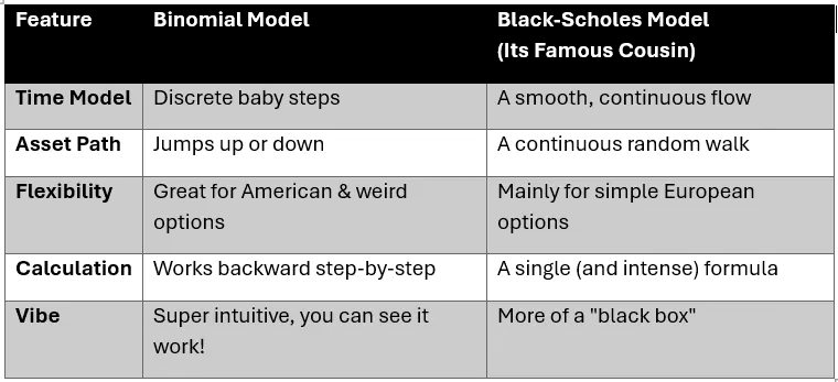
In fact, the binomial model is the discrete, step-by-step version of the most famous formula in finance: the Black-Scholes model. As you add more and more steps to your binomial tree, the price you get gets closer and closer to the Black-Scholes price. They are two sides of the same coin. Given below is comparison between the two:

By building this from the ground up, you’ve gained something more valuable than a formula: an intuition for how replication, hedging, and risk-neutral valuation work.

The logic of the Matrix is now clear. Go forth and price things!