Decision Trees, Ensembles, and Advanced Boosting Techniques

Introduction

In last part, we explored Bayesian methods which rely on probability theory and the assumption of feature independence. While powerful, financial data often contains complex, non-linear interactions that simple independence assumptions cannot capture. For instance, a high P/E ratio might be bad for a utility stock but acceptable for a tech stock; the effect of one variable depends on the value of another.

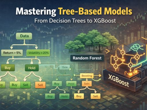
This brings us to Decision Trees and their powerful evolution into Ensemble Methods like Random Forests and Gradient Boosting (XGBoost). These algorithms mimic human decision-making by splitting data into smaller, more homogeneous groups based on a series of questions.

Section 1: The Anatomy of a Decision Tree

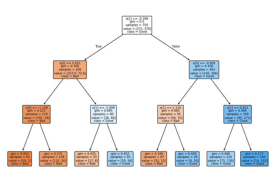
A decision tree is a flowchart-like structure used for both classification and regression. It allows us to segment the predictor space into regions.

1.1 Components of the Tree

• Root Node: The very top of the tree. This node contains the entire dataset before any splits are made.
• Interior Nodes (Decision Nodes): These are nodes where a split occurs based on a specific feature condition (e.g., “Is Return > 5%?”).
• Branches: The arrows connecting nodes, representing the outcome of the decision (True/False).
• Leaf Nodes (Terminal Nodes): The final nodes at the bottom of the tree. These nodes do not split further and contain the final prediction (e.g., Class: “Buy”).

1.2 How Trees “Learn” (Splitting Criteria)

The core logic of a decision tree is determining the best question to ask at each node. “Best” is defined as the split that results in the highest purity or homogeneity in the resulting child nodes.

For classification, we use metrics like Gini Impurity or Entropy.

Gini Impurity:

Gini measures the likelihood of an incorrect classification of a new instance of a random variable, if that new instance were randomly classified according to the distribution of class labels from the dataset.

Formula for a node with $C$ classes:

$$ Gini = 1 – sum_{i=1}^{C} (p_i)^2 $$

Where $p_i$ is the probability of an item belonging to class $i$.

1. A Gini of 0.0 means the node is “pure” (all samples belong to one class).
2. A Gini of 0.5 (for binary classification) implies a random 50/50 mix.

Information Gain (Entropy):

Entropy measures the amount of disorder or uncertainty.

$$ Entropy = – sum_{i=1}^{C} p_i log_2(p_i) $$

The algorithm calculates the weighted average impurity of potential splits and chooses the one that reduces impurity the most (Information Gain).

Section 2: Regularization and Pruning

Decision trees have a major weakness: Overfitting. A tree can grow indefinitely, creating a specific leaf node for every single outlier in the training data. This creates a model that memorizes the training set but fails on new data (high variance).

To combat this, we use Pruning:

• Pre-Pruning (Early Stopping): We stop the tree from growing before it becomes too complex.
  • max_depth: Limit how deep the tree can go.
  • min_samples_split: Require a minimum number of samples to create a split.
  • min_samples_leaf: Require a minimum number of samples in a terminal node.
• Post-Pruning (Cost-Complexity Pruning): We grow the full tree and then cut back branches that add little predictive power relative to their complexity.

Section 3: Ensemble Methods and Boosting

While a single tree is prone to high variance, Ensemble Learning combines multiple trees to create a robust model.

3.1 Bagging vs. Boosting

• Bagging (Bootstrap Aggregating): Builds many independent trees in parallel on random subsets of data and averages their predictions (e.g., Random Forest). This reduces variance.
• Boosting: Builds trees sequentially. Each new tree focuses on correcting the errors made by the previous trees. This reduces bias and variance.

3.2 AdaBoost (Adaptive Boosting)

AdaBoost was the first successful boosting algorithm. It works by assigning weights to data points.

1. Train a weak decision tree (a “stump”).
2. Identify the misclassified points.
3. Increase the weight of misclassified points so the next tree focuses harder on them.
4. Repeat.

The final prediction is a weighted vote of all trees.

3.3 Gradient Boosting and XGBoost

Gradient Boosting takes a different approach. Instead of updating weights, it trains the new tree to predict the residuals (errors) of the previous tree.

$$ Prediction_{new} = Prediction_{old} + LearningRate times Error $$

XGBoost (Extreme Gradient Boosting) is an optimized implementation of this concept widely used in finance for its speed and performance. It introduces:

• Regularization: Built-in L1 and L2 regularization to prevent overfitting.
• Sparsity Handling: Handles missing data automatically.
• Parallel Processing: Much faster training than standard Gradient Boosting.

Section 4: Model Evaluation Metrics

In financial classification, simple accuracy is often misleading (e.g., in a fraud dataset where 99% of cases are legitimate, predicting “legitimate” every time gives 99% accuracy but is useless).

4.1 ROC Curve and AUC

We use the Receiver Operating Characteristic (ROC) curve.

1. X-axis: False Positive Rate (1 – Specificity).
2. Y-axis: True Positive Rate (Sensitivity/Recall).

The curve visualizes the trade-off between capturing positives and flagging false alarms at various threshold settings.

AUC (Area Under the Curve):

A single number summary of the ROC.

• AUC = 0.5: Random guessing.
• AUC = 1.0: Perfect classifier.
• AUC > 0.7: Generally considered good.

There is a mathematical relationship between the Gini coefficient (from economics) and AUC:

$$ Gini_2 = 2 times AUC – 1 $$

(Note: This Gini is distinct from Gini Impurity used in splitting).

Section 5: Practical Implementation (Decision Trees & XGBoost)

We will now implement a Decision Tree and an XGBoost classifier using Python.

5.1 Data Preparation

We assume X_train, X_test, y_train, and y_test are already defined (as in last part).

5.2 Implementing a Single Decision Tree

We use sklearn.tree.DecisionTreeClassifier.

from sklearn.tree import DecisionTreeClassifier

from sklearn import tree

import matplotlib.pyplot as plt

 

# Initialize tree with pre-pruning to prevent overfitting

dt_model = DecisionTreeClassifier(

criterion=‘gini’, # Splitting criteria

max_depth=3, # Limit depth

min_samples_leaf=5, # Min samples in leaf

random_state=42

)

 

dt_model.fit(X_train, y_train)

 

# Visualize the tree

plt.figure(figsize=(12,8))

tree.plot_tree(dt_model, filled=True, rounded=True, class_names=[‘Bad’, ‘Good’])

plt.show()

 

# Evaluate

dt_pred = dt_model.predict(X_test)

print(“Decision Tree Accuracy:”, accuracy_score(y_test, dt_pred))

 

5.3 Implementing XGBoost

We use the xgboost library. This is the industry standard for tabular data in finance.

from xgboost import XGBClassifier

# Initialize XGBoost

# n_estimators: Number of trees (boosting rounds)

# learning_rate: Step size shrinkage to prevent overfitting

# max_depth: Depth of individual trees

xgb_model = XGBClassifier(

n_estimators=100,

learning_rate=0.1,

max_depth=3,

use_label_encoder=False,

eval_metric=‘logloss’

)

 

xgb_model.fit(X_train, y_train)

 

# Predictions

xgb_pred = xgb_model.predict(X_test)

print(“XGBoost Accuracy:”, accuracy_score(y_test, xgb_pred))

 

5.4 Feature Importance

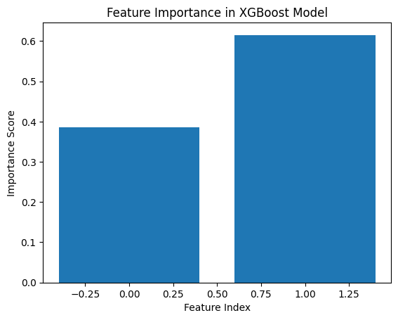
One of the advantages of tree-based models is interpretability via feature importance.

# Extract feature importance

importances = xgb_model.feature_importances_

 

# Plotting

plt.bar(range(len(importances)), importances)

plt.title(“Feature Importance in XGBoost Model”)

plt.xlabel(“Feature Index”)

plt.ylabel(“Importance Score”)

plt.show()

 

Conclusion

In this part, we moved from the independence assumptions of Bayesian statistics to the hierarchical decision-making of Trees. We explored how a single tree splits data based on purity, how ensembles like Boosting fix the weaknesses of single trees, and how XGBoost acts as a robust tool for financial classification.

By mastering both Bayesian and Tree-based methods, a financial data scientist is equipped with tools for both probabilistic inference (Bayes) and high-accuracy non-linear prediction (XGBoost).