Machine Learning for Quants Series with Python (Part 9)

Introduction

In Part 8, we explored parallel ensemble methods. In Bagging and Stacking, our base models are largely independent; the SVM doesn’t know or care what the Decision Tree is doing.

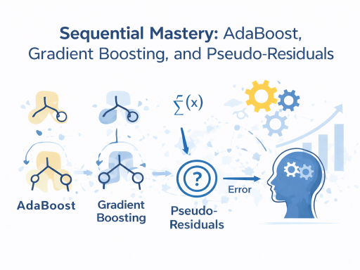
Boosting flips this paradigm entirely. Boosting is a sequential process. It builds a model, evaluates where that model failed, and then builds a new model explicitly designed to fix the mistakes of the previous one.

In this tutorial, we will demystify the two most famous boosting algorithms: AdaBoost (Adaptive Boosting) and Gradient Boosting. We will apply them to a common banking risk problem: predicting Credit Card Defaults, highlighting how these algorithms iteratively hunt down difficult-to-predict outliers.

Learning Objectives

By the end of this tutorial, you will be able to:

1. Explain the mechanics of AdaBoost, specifically “Sampling with Replacement” driven by dynamic sample weights and “Amount of Say.”
2. Define “Pseudo-Residuals” and explain how Gradient Boosting fits trees to the loss gradient rather than the target variable.
3. Tune crucial boosting hyperparameters, specifically the inverse relationship between learning_rate and n_estimators.
4. Compare the performance characteristics of Bagged vs. Boosted models.

Prerequisites

1. Prior Knowledge: Decision Trees, Ensemble methodology, Basics of Loss Functions.
2. Libraries: scikit-learn, pandas, numpy, matplotlib.

Core Concepts

1. AdaBoost: The “Amount of Say”

AdaBoost uses very short Decision Trees called “Stumps” (a tree with a depth of 1, meaning it only makes a single split).

Here is how it learns sequentially:

1. Initialize Weights: Every data point starts with an equal weight.
2. Train a Stump: A stump is trained to minimize the weighted error.
3. Calculate “Amount of Say”: The algorithm calculates how accurate the stump was. Highly accurate stumps get a large “Amount of Say” (voting power) in the final ensemble.
4. Update Sample Weights: Crucial Step. The algorithm increases the weight of the data points the stump got wrong, and decreases the weight of the ones it got right.
5. Repeat: The next stump is trained. Because the weights have changed, this new stump is mathematically forced to focus on the difficult points the previous stump missed.

2. Gradient Boosting: Fitting to the Error

Gradient Boosting (GBM) takes a more advanced, calculus-based approach. It doesn’t use sample weights. Instead, it alters the target variable for the next tree.

• Initial Prediction: It starts with a naive prediction (like the average value of all targets).
• Calculate Pseudo-Residuals: It calculates the difference between the actual value and the predicted value (the error, or “residual”). In calculus terms, this residual is the negative gradient of the Mean Squared Error loss function.
• Train a Tree on the Residuals: It trains a new decision tree, but the target y is no longer “Default” or “No Default”. The target y is now the residual value. The tree is learning how much to adjust the previous prediction.
• Combine and Apply Learning Rate: The new tree’s predictions are multiplied by a small learning_rate and added to the cumulative prediction.

The Hands-On Practice

Step 1: Loading the Credit Default Dataset

We will use a synthetic dataset designed to mimic the famous UCI Credit Card Default dataset, focusing on predicting whether a client will default based on payment history and balances.

import numpy as np

import pandas as pd

import matplotlib.pyplot as plt

from sklearn.datasets import make_classification

from sklearn.model_selection import train_test_split

from sklearn.metrics import classification_report, roc_auc_score

 

# Simulate Credit Card Default Data

# Defaults are often imbalanced; we set weights to 80% non-default, 20% default

X, y = make_classification(n_samples=3000, n_features=15, n_informative=10,

weights=[0.8, 0.2], random_state=42)

 

X_train, X_test, y_train, y_test = train_test_split(X, y, test_size=0.25, random_state=42)

 

print(f“Target Distribution in Train: {np.bincount(y_train)}”)

 

Step 2: Implementing AdaBoost

We will use AdaBoostClassifier from scikit-learn. By default, it uses Decision Tree Stumps as its base estimator.

from sklearn.ensemble import AdaBoostClassifier

 

# Initialize AdaBoost

# n_estimators: The maximum number of stumps to build

# learning_rate: Shrinks the contribution of each classifier

ada_model = AdaBoostClassifier(n_estimators=50, learning_rate=1.0, random_state=42)

 

# Train the model

ada_model.fit(X_train, y_train)

 

# Predict and Evaluate

ada_pred = ada_model.predict(X_test)

ada_prob = ada_model.predict_proba(X_test)[:, 1]

 

print(“— AdaBoost Performance —“)

print(classification_report(y_test, ada_pred))

print(f“AdaBoost AUC: {roc_auc_score(y_test, ada_prob):.4f}”)

 

Step 3: Implementing Gradient Boosting

Now we implement GradientBoostingClassifier. Notice how the hyperparameters change. We use deeper trees (usually depth 3-5) rather than stumps.

from sklearn.ensemble import GradientBoostingClassifier

 

# Initialize Gradient Boosting

# max_depth: GBMs use slightly deeper trees than AdaBoost’s stumps

gb_model = GradientBoostingClassifier(n_estimators=100, learning_rate=0.1,

max_depth=3, random_state=42)

 

# Train the model

gb_model.fit(X_train, y_train)

 

# Predict and Evaluate

gb_pred = gb_model.predict(X_test)

gb_prob = gb_model.predict_proba(X_test)[:, 1]

 

print(“n— Gradient Boosting Performance —“)

print(classification_report(y_test, gb_pred))

print(f“Gradient Boosting AUC: {roc_auc_score(y_test, gb_prob):.4f}”)

 

Step 4: The Learning Rate Trade-off (Trainer Deep Dive)

In Gradient Boosting, the prediction of the ensemble at step M is:

Fmx=Fm-1x+ν⋅hmx

Where ν is the learning_rate and hmx is the new tree.

Note:: There is a perfect inverse relationship between learning_rate and n_estimators. If you drop the learning rate from 0.1 to 0.01, the model takes smaller steps. To reach the same predictive power, it will need 10 times as many trees (n_estimators). Smaller learning rates generally lead to better generalization (less overfitting) but take longer to train.

# Demonstrating the trade-off visually by plotting training deviance (loss)

train_errors_high_lr = []

train_errors_low_lr = []

 

# High LR model (0.5)

gb_high = GradientBoostingClassifier(n_estimators=100, learning_rate=0.5, random_state=42)

gb_high.fit(X_train, y_train)

 

# Low LR model (0.05)

gb_low = GradientBoostingClassifier(n_estimators=100, learning_rate=0.05, random_state=42)

gb_low.fit(X_train, y_train)

 

# Plotting the loss at each boosting stage

plt.figure(figsize=(10, 5))

plt.plot(gb_high.train_score_, label=‘High Learning Rate (0.5)’, color=‘red’)

plt.plot(gb_low.train_score_, label=‘Low Learning Rate (0.05)’, color=‘blue’)

plt.title(“Gradient Boosting: Loss vs. Boosting Iterations”)

plt.xlabel(“Number of Trees (n_estimators)”)

plt.ylabel(“Loss (Deviance)”)

plt.legend()

plt.grid(True)

plt.show()

 

Observation: The high learning rate model drops its loss rapidly but risks overshooting the optimal solution (and often overfits). The low learning rate model descends smoothly and steadily, indicating a more stable learning process.

Check Your Work:

• AdaBoost vs. Random Forest: How does AdaBoost’s approach to difficult data points differ from Random Forest? (Answer: Random Forest hopes that by sheer chance, some trees will catch the outliers. AdaBoost mathematically forces later trees to focus entirely on the outliers).
• Loss Functions: By default, GradientBoostingClassifier uses ‘log_loss’ (Deviance) for classification. If we were predicting continuous returns (Regression), it would use Least Squares error, and the pseudo-residuals would exactly equal Actual – Predicted.

Conclusion

We have now mastered sequential ensemble learning. We explored how AdaBoost intelligently adjusts the weight of historical data to force weak learners to become stronger collectively. We then examined Gradient Boosting, a mathematically elegant approach that uses numerical optimization (gradient descent) to iteratively fit trees to the errors of previous trees.

Understanding pseudo-residuals, loss functions, and learning rates forms the absolute bedrock of modern tabular machine learning. In the real quantitative industry, advanced frameworks like XGBoost, LightGBM, and CatBoost are all built directly upon the Gradient Boosting principles we established in this lesson.