Machine Learning for Quants Series with Python (Part 11)

Introduction

In previous modules, we explored probabilistic models (Naive Bayes) and hierarchical algorithms (Decision Trees and Ensembles). While tree-based models excel at slicing data into rectangular regions, financial markets often exhibit continuous, non-linear boundaries between profitable and unprofitable regimes.

Enter the Support Vector Machine (SVM). Originally developed in the 1990s, the SVM is a mathematically elegant algorithm designed to find the optimal boundary (the hyperplane) that separates different classes of data.

In this tutorial, we will explore the geometric intuition behind SVMs. We will learn how to maximize the “Margin,” how to handle noisy financial data using “Slack Variables,” and how to use the “Kernel Trick” to project non-linear market data into higher dimensions where linear separation becomes possible.

Learning Objectives

By the end of this tutorial, you will be able to:

• Explain the geometric concept of Hyperplanes, Margins, and Support Vectors.
• Differentiate between Hard Margins and Soft Margins (using the hyperparameter C / Slack Variables).
• Understand the Kernel Trick and its application to non-linear financial data.
• Implement an SVM trading strategy in Python to predict long positions of an index, evaluating it with ROC and AUC.

Prerequisites

1. Prior Knowledge: Classification metrics, Training/Testing splits, Feature Scaling (Crucial for SVMs).
2. Libraries: scikit-learn, pandas, numpy, matplotlib.

Core Concepts

1. The Hyperplane and the Margin

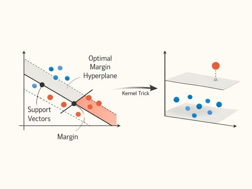
Imagine a 2D scatter plot where blue dots represent “Up” days and red dots represent “Down” days. A hyperplane is simply a line that separates the blue dots from the red dots. (In 3D, it’s a flat plane; in higher dimensions, it’s a hyperplane).

An infinite number of lines could separate the data. The genius of the SVM is that it doesn’t just find any line; it finds the Optimal Margin Hyperplane.

• The Margin is the distance between the hyperplane and the closest data points from either class.
• Support Vectors are those exact closest data points. They are the only points that actually matter to the model; if you removed all other data points, the hyperplane would not change. The model is “supported” entirely by these critical edge cases.

2. Soft Margins and Slack Variables (Handling Market Noise)

In financial markets, perfect separation is impossible. Data is noisy, and anomalies occur. If an SVM tries to perfectly separate every single point (a Hard Margin), it will overfit drastically to outliers.

To fix this, we introduce Slack Variables (ξ). Slack allows certain points to be on the wrong side of the margin (or even the wrong side of the hyperplane) without breaking the model.

• The C Hyperparameter: This controls the penalty for slack.
  • A High C strictly penalizes errors, leading to a narrower margin and potential overfitting (Hard Margin).
  • A Low C is more forgiving, allowing more violations in exchange for a wider, more generalized margin (Soft Margin).

3. The Kernel Trick (Non-Linearity)

What if the blue and red dots are arranged in a circle, meaning no straight line can separate them?

The Kernel Trick is a mathematical shortcut. Instead of drawing a curved line, a Kernel function mathematically projects the 2D data into a 3D space (e.g., pulling the center points upwards). In this new 3D space, we can easily slice a flat, straight plane through the data to separate it.

• Common Kernels: Linear, Polynomial, and RBF (Radial Basis Function – the default, highly effective for complex, non-linear relationships).

Trainer’s Tip: Imagine drawing a red dot on a sheet of paper surrounded by a ring of blue dots. You cannot draw a straight line separating them. Now imagine placing a marble under the paper at the red dot. The paper bulges up in the 3rd dimension. You can now easily slice the top of the bulge (red) off from the rest of the paper (blue) with a perfectly flat 2D plane!

The Hands-On Practice

Step 1: Data Preparation and Feature Scaling

We will simulate technical indicator data for an index to predict whether taking a long position will be profitable.

import numpy as np

import pandas as pd

import matplotlib.pyplot as plt

from sklearn.datasets import make_classification

from sklearn.model_selection import train_test_split

from sklearn.preprocessing import StandardScaler

from sklearn.svm import SVC

from sklearn.metrics import accuracy_score, classification_report, roc_curve, auc

 

# Simulate Financial Market Data (1500 days, 5 technical indicators)

X, y = make_classification(n_samples=1500, n_features=5, n_informative=3,

n_redundant=1, random_state=42, class_sep=0.8)

 

X_train, X_test, y_train, y_test = train_test_split(X, y, test_size=0.2, random_state=42)

 

# CRITICAL STEP: Scaling

# SVMs optimize geometric distance. If one indicator ranges from 1-100 and another from 0-0.01,

# the large numbers will dominate the distance calculation mathematically.

scaler = StandardScaler()

X_train_scaled = scaler.fit_transform(X_train)

X_test_scaled = scaler.transform(X_test)

 

Step 2: Training the Support Vector Classifier (SVC)

We will initialize an SVC using the default RBF kernel and a balanced C parameter.

# Initialize the SVM Classifier

# probability=True allows us to plot ROC curves later

svm_model = SVC(kernel=‘rbf‘, C=1.0, probability=True, random_state=42)

 

# Train the model

print(“Training SVM Model…”)

svm_model.fit(X_train_scaled, y_train)

 

# Predict

y_pred = svm_model.predict(X_test_scaled)

 

print(“— SVM Performance —“)

print(classification_report(y_test, y_pred))

 

Step 3: Visualizing the ROC Curve

To compare this model against a random guess, we plot the Receiver Operating Characteristic (ROC) curve.

# Get prediction probabilities for Class 1 (Long Position)

y_prob = svm_model.predict_proba(X_test_scaled)[:, 1]

 

fpr, tpr, thresholds = roc_curve(y_test, y_prob)

roc_auc = auc(fpr, tpr)

 

plt.figure(figsize=(8, 6))

plt.plot(fpr, tpr, color=‘blue’, lw=2, label=f‘SVM ROC curve (AUC = {roc_auc:.2f})’)

plt.plot([0, 1], [0, 1], color=‘red’, linestyle=‘–‘, label=‘Random Guess’)

plt.xlabel(‘False Positive Rate’)

plt.ylabel(‘True Positive Rate’)

plt.title(‘SVM ROC Curve for Index Long Strategy’)

plt.legend(loc=“lower right”)

plt.grid(True)

plt.show()

 

Check Your Work:

• Scaling Validation: Try running svm_model.fit(X_train, y_train) (without the scaled data). You will likely see execution times increase and accuracy drop significantly. This reinforces why scaling is non-negotiable for margin-based algorithms.
• Hyperparameter Tuning: Write a loop to train the SVM with C values of [0.01, 1, 100]. Observe how the training accuracy vs. testing accuracy shifts, illustrating the transition from High Bias (Underfitting) to High Variance (Overfitting).

Conclusion

In this part, we explored the mathematical elegance of Support Vector Machines. We learned how SVMs seek the Optimal Margin Hyperplane, how slack variables prevent the model from obsessing over financial noise, and how the Kernel trick handles complex, non-linear market realities.

SVMs are powerful, robust to overfitting (especially in high-dimensional spaces), and highly effective for classification tasks. However, as datasets grow to millions of rows, SVM training times can become computationally prohibitive. This brings us to the next massive leap in modern quantitative analysis: Artificial Neural Networks.