Machine Learning for Quants Series with Python (Part 12)

Introduction

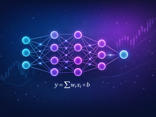
We have reached the frontier of modern machine learning: Deep Learning. While SVMs and Ensembles define “Classical ML”, Artificial Neural Networks (ANNs) mimic the architecture of the human brain to learn representations of data with multiple levels of abstraction.

In quantitative finance, ANNs are used for complex tasks where traditional feature engineering fails: high-frequency trading pattern recognition, natural language processing on earnings transcripts, and modeling non-linear macroeconomic relationships.

In this tutorial, we will break down the biological inspiration of the Neuron into mathematical equations. We will explore Forward Propagation, Loss Functions, and Backpropagation. Finally, we will build a Neural Network regression model using Keras and TensorFlow to predict continuous economic data.

Learning Objectives

By the end of this tutorial, you will be able to:

1. Explain the architecture of a Neural Network: Neurons, Weights, Biases, and Hidden Layers.
2. Understand the role of Activation Functions (introducing non-linearity) and Optimizers (Gradient Descent).
3. Identify common Deep Learning pitfalls like Vanishing Gradients and Overfitting.
4. Build and compile a deep neural network using Keras/TensorFlow to predict continuous variables using Mean Squared Error (MSE) and Mean Absolute Error (MAE).

Prerequisites

• Prior Knowledge: Linear algebra basics, Gradient Descent concept, Feature Scaling.
• Libraries: scikit-learn, pandas, numpy, matplotlib, tensorflow, keras.

Core Concepts

1. The Perceptron (The Artificial Neuron)

At the core of an ANN is the neuron. Mathematically, a neuron receives multiple inputs (X), multiplies each by a specific Weight (w), adds a constant Bias (b), and passes the result through an Activation Function.

Z=w1x1+w2x2+…+wnxn+b

Output = ActivationFunction(Z)

2. The Network Architecture

• Input Layer: The raw financial data (e.g., 10 technical indicators means 10 input nodes).
• Hidden Layers: The layers between input and output. A network with more than one hidden layer is considered “Deep Learning.” Each node in a hidden layer connects to every node in the previous layer (a “Dense” layer).
• Output Layer: The final prediction. For regression (predicting a return), this is typically a single node with a linear activation function.

3. Forward Propagation vs. Backpropagation

• Forward Propagation: Data flows from input to output. The network makes a prediction.
• The Loss Function: The network compares its prediction to the actual truth. For financial regression, we use Mean Squared Error (MSE) or Mean Absolute Error (MAE).
• Backpropagation: The “learning” phase. Using calculus (the chain rule), the network calculates the gradient of the loss function with respect to every single weight. It then sends an error signal backward through the network, updating the weights to minimize the loss.
• The Optimizer: Algorithms like SGD (Stochastic Gradient Descent) or Adam dictate how the weights are updated based on those gradients.

4. Pitfalls: Overfitting and Vanishing Gradients

• Overfitting: Because ANNs have thousands (or millions) of parameters, they can easily memorize noise.
• Vanishing Gradients: As the error signal travels backward through many deep layers, the gradient can shrink to near-zero, meaning the earliest layers stop learning. Modern activation functions (like ReLU) solve this.

Trainer’s Tip: Backpropagation is like a game of “Telephone” combined with a blame game. The output node realizes it made a mistake. It looks at the nodes feeding into it and adjusts their weights based on who contributed most to the error. Those nodes then turn around and adjust the weights of the nodes behind them, propagating the correction all the way back to the inputs.

The Hands-On Practice

Step 1: Data Preparation

We will simulate continuous economic data to predict an asset’s future return (a Regression problem).

import numpy as np

import pandas as pd

import matplotlib.pyplot as plt

from sklearn.model_selection import train_test_split

from sklearn.preprocessing import StandardScaler

import tensorflow as tf

from tensorflow.keras.models import Sequential

from tensorflow.keras.layers import Dense

 

# Simulate Continuous Economic Data (2000 samples, 8 macroeconomic factors)

np.random.seed(42)

tf.random.set_seed(42)

 

X = np.random.randn(2000, 8)

# Target y is a complex non-linear combination of the inputs + noise

y = (np.sin(X[:, 0]) + X[:, 1]**2 + np.log(np.abs(X[:, 2])+1) – X[:, 3]*1.5) + np.random.normal(0, 0.5, 2000)

 

X_train, X_test, y_train, y_test = train_test_split(X, y, test_size=0.2, random_state=42)

 

# Neural Networks are EXTREMELY sensitive to unscaled data

scaler = StandardScaler()

X_train_scaled = scaler.fit_transform(X_train)

X_test_scaled = scaler.transform(X_test)

 

Step 2: Building the Architecture using Keras

We use the Sequential API to stack layers. We will build a deep network with two hidden layers. We use the ReLU (Rectified Linear Unit) activation function for hidden layers to prevent vanishing gradients.

# Initialize a Sequential model

model = Sequential()

 

# Add the first Hidden Layer (requires input_dim matching feature count)

# 64 neurons, ReLU activation

model.add(Dense(64, activation=‘relu’, input_dim=X_train_scaled.shape[1]))

 

# Add a second Hidden Layer

# 32 neurons, ReLU activation

model.add(Dense(32, activation=‘relu’))

 

# Add the Output Layer

# 1 neuron, Linear activation (default) because we are predicting a continuous numerical value

model.add(Dense(1))

 

# Review the architecture

model.summary()

 

Step 3: Compiling the Model

Compiling defines how the model will learn.

• Loss: mse (Mean Squared Error).
• Optimizer: adam (An advanced version of gradient descent that adapts the learning rate automatically).
• Metrics: We track mae (Mean Absolute Error) for human readability (e.g., “The model is off by an average of 1.5 units”).

model.compile(optimizer=‘adam’, loss=‘mse’, metrics=[‘mae’])

 

Step 4: Training the Network (Epochs and Batch Size)

• Epochs: How many times the model sees the entire dataset.
• Batch Size: How many rows the model processes before updating its weights. Smaller batches introduce beneficial noise to the learning process and require less memory.

# Train the model

history = model.fit(

X_train_scaled, y_train,

epochs=50,

batch_size=32,

validation_split=0.2, # Hold out 20% of training data to check for overfitting

verbose=0 # Set to 1 to see the progress bar

)

 

print(“Training Complete.”)

 

Step 5: Visualizing Learning and Evaluating

We plot the loss curve to ensure the model actually learned and didn’t overfit.

# Plot Training vs. Validation Loss

plt.figure(figsize=(10, 5))

plt.plot(history.history[‘loss’], label=‘Training Loss (MSE)’)

plt.plot(history.history[‘val_loss’], label=‘Validation Loss (MSE)’)

plt.title(‘Neural Network Learning Curve’)

plt.xlabel(‘Epochs’)

plt.ylabel(‘Mean Squared Error’)

plt.legend()

plt.grid(True)

plt.show()

 

# Final Evaluation on the unseen Test Set

test_loss, test_mae = model.evaluate(X_test_scaled, y_test, verbose=0)

print(f“Test Set Final MSE: {test_loss:.4f}”)

print(f“Test Set Final MAE: {test_mae:.4f}”)

 

Check Your Work:

• Learning Curve Analysis: Look at the plot generated in Step 5. If the Training Loss goes down, but the Validation Loss starts going up after epoch 20, the model is overfitting! (Solution: Stop training earlier, a technique called “Early Stopping”).
• Architecture Tinkering: Change the output activation from linear (default) to activation=’sigmoid’. Notice how the model completely fails? A sigmoid forces outputs between 0 and 1, but our target y ranges from roughly -5 to +5. The output layer activation must match your target distribution!

Conclusion

In this part, we crossed into the realm of Deep Learning. We learned that Artificial Neural Networks are essentially massive arrays of mathematical functions interconnected by learnable weights. We used Keras and TensorFlow to define layers, select loss functions (MSE), and apply backpropagation via the Adam optimizer to model complex economic regressions.

While ANNs are incredibly powerful, they are “black boxes.” Unlike Decision Trees or Linear Regression, explaining why a neural network decided to buy a stock is immensely difficult. In quantitative finance, balancing predictive accuracy with model interpretability remains one of the greatest challenges for practitioners.