Machine Learning for Quants Series with Python (Part 13)

Introduction

In Part 12, we built our first Artificial Neural Network (ANN). We defined the architecture (neurons, layers, and activation functions) and briefly touched upon backpropagation. However, knowing the architecture of a car engine is different from understanding the fuel combustion that actually drives it forward.

In Deep Learning, that “fuel” is Optimization. How exactly does a network with hundreds of thousands of random initial weights find the specific combination that accurately predicts financial markets?

In this tutorial, we will dive into the mathematics of optimization. We will explore the topography of Loss Landscapes, the difference between Convex and Non-Convex functions, and the mechanics of Gradient Descent; specifically why Stochastic Gradient Descent (SGD) is the absolute lifeblood of modern Deep Learning.

Learning Objectives

By the end of this tutorial, you will be able to:

• Visualize and explain the difference between Convex and Non-Convex optimization problems.
• Understand the mathematical mechanics of Gradient Descent and how it uses the derivative (gradient) to find minimum error.
• Differentiate between Batch Gradient Descent, Stochastic Gradient Descent (SGD), and Mini-Batch SGD.
• Implement and compare different optimization strategies in Python to see their impact on training speed and convergence.

Prerequisites

1. Prior Knowledge: Neural Network Architecture, Basic Calculus (Concept of a Derivative/Slope).
2. Libraries: scikit-learn, numpy, matplotlib, tensorflow, keras.

Core Concepts

1. The Loss Landscape: Convexity vs. Non-Convexity

When we train a neural network, we are trying to find the lowest possible point (minimum error) on a multidimensional surface called the Loss Landscape.

• Convex Functions: Imagine a smooth, simple bowl. If you drop a marble anywhere in the bowl, gravity pulls it directly to the singular lowest point at the bottom. Linear Regression and Logistic Regression have convex loss functions. They are easy to optimize because there is only one global minimum.
• Non-Convex Functions: Deep Neural Networks are highly non-linear, creating a landscape that looks like a rugged mountain range with many peaks and valleys. If you drop a marble here, it might get stuck in a shallow valley (a Local Minimum) and never reach the true bottom (the Global Minimum).

Trainer’s Tip: You are blindfolded on a mountain and want to reach the absolute lowest valley. You can only feel the slope of the ground right under your feet. If you just step downhill, you might end up at the bottom of a crater halfway up the mountain (Local Minimum), completely missing the valley floor.

2. Gradient Descent

Gradient Descent is the algorithm that tells our “blindfolded hiker” which way to step.

• It calculates the Gradient (the slope or derivative) of the loss function with respect to the weights.
• It takes a step in the opposite direction of the gradient (downhill).
• The size of the step is controlled by the Learning Rate ($alpha$).
  • If $alpha$ is too small, training takes forever.
  • If $alpha$ is too large, the model might “jump over” the valley and diverge completely.

3. Batch vs. Stochastic vs. Mini-Batch

Calculating the true gradient requires looking at the entire dataset before taking a single step.

• Batch Gradient Descent: Uses the whole dataset. It is precise, but incredibly slow, and prone to getting stuck in local minima because the landscape never changes.
• Stochastic Gradient Descent (SGD): Uses one single data point to estimate the gradient and takes a step. It is chaotic and highly noisy, but this “noise” allows it to bounce out of local minima!
• Mini-Batch SGD: The industry standard. It uses a small, random subset of data (e.g., 32 or 64 samples) for each step. It balances the computational efficiency of Batch with the beneficial noise of Stochastic.

The Hands-On Practice

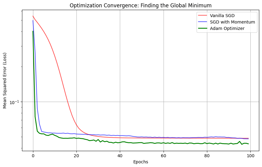
Let’s visualize how different optimization algorithms converge using Keras. We will simulate a noisy financial regression task and train the exact same network architecture using three different optimizers: Standard SGD, SGD with Momentum, and Adam.

import numpy as np

import matplotlib.pyplot as plt

import tensorflow as tf

from tensorflow.keras.models import Sequential

from tensorflow.keras.layers import Dense

from tensorflow.keras.optimizers import SGD, Adam

 

# 1. Simulate a complex, non-linear financial dataset

np.random.seed(42)

tf.random.set_seed(42)

X = np.random.uniform(-5, 5, (1000, 1))

# Target is a sine wave with noise (highly non-convex relationship)

y = np.sin(X) + np.random.normal(0, 0.2, (1000, 1))

 

# Function to build our standard architecture

def build_model(optimizer):

model = Sequential([

Dense(32, activation=‘relu’, input_shape=(1,)),

Dense(32, activation=‘relu’),

Dense(1) # Linear output for regression

])

model.compile(optimizer=optimizer, loss=‘mse’)

return model

 

# 2. Define Optimizers to Compare

# Vanilla SGD (Often slow and gets stuck)

opt_sgd = SGD(learning_rate=0.01)

 

# SGD with Momentum (Builds up speed in consistent directions)

opt_momentum = SGD(learning_rate=0.01, momentum=0.9)

 

# Adam (Adaptive Moment Estimation – Industry Standard)

opt_adam = Adam(learning_rate=0.01)

 

# 3. Train the Models

epochs = 100

batch_size = 32 # Using Mini-Batch approach

 

print(“Training Vanilla SGD…”)

history_sgd = build_model(opt_sgd).fit(X, y, epochs=epochs, batch_size=batch_size, verbose=0)

 

print(“Training SGD with Momentum…”)

history_momentum = build_model(opt_momentum).fit(X, y, epochs=epochs, batch_size=batch_size, verbose=0)

 

print(“Training Adam…”)

history_adam = build_model(opt_adam).fit(X, y, epochs=epochs, batch_size=batch_size, verbose=0)

 

# 4. Plot the Loss Convergence

plt.figure(figsize=(10, 6))

plt.plot(history_sgd.history[‘loss’], label=‘Vanilla SGD’, color=‘red’, alpha=0.7)

plt.plot(history_momentum.history[‘loss’], label=‘SGD with Momentum’, color=‘blue’, alpha=0.7)

plt.plot(history_adam.history[‘loss’], label=‘Adam Optimizer’, color=‘green’, linewidth=2)

plt.title(‘Optimization Convergence: Finding the Global Minimum’)

plt.xlabel(‘Epochs’)

plt.ylabel(‘Mean Squared Error (Loss)’)

plt.legend()

plt.yscale(‘log’) # Log scale helps visualize the rapid drop

plt.grid(True)

plt.show()

 

Check Your Work:

• Observe the Convergence: Notice how Vanilla SGD drops slowly and plateaus. Adam (which dynamically adjusts the learning rate for every single weight) drops like a stone. Momentum sits somewhere in between.
• Tweak the Batch Size: Change batch_size=32 to batch_size=1000 (Full Batch). Watch how slowly the model learns per epoch because it only takes one step per epoch!

Conclusion

Understanding optimization separates practitioners who just copy-paste code from true quantitative developers. Because Deep Learning loss landscapes are non-convex, you cannot rely on simple math to find the absolute truth. You must rely on clever navigation strategies like Mini-Batch SGD, Momentum, and Adam to traverse the mountains and find the deepest valley.

In the next part, we will take our perfectly optimized Neural Networks and apply them to two of the most critical domains in finance: Modeling the Yield Curve and Predicting Credit Defaults using advanced balancing techniques like SMOTE.

<br>