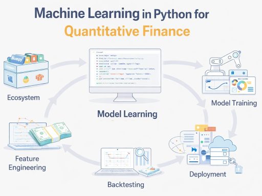
Welcome to the comprehensive guide on building Machine Learning (ML) solutions for quantitative finance using Python. Whether you are transitioning from traditional econometrics, stepping into algorithmic trading, or building risk models, understanding both your tools and the rigorous process is non-negotiable.

In finance, a poorly implemented model doesn’t just give a bad recommendation; it loses money. Many junior quants make the mistake of diving straight into complex deep learning algorithms without understanding the underlying ecosystem or the strict methodology required to build models that survive out-of-sample in real markets.

In this detailed, step-by-step guide, we will break down the journey into two distinct parts:

• The Python ML Ecosystem: The essential packages and libraries you need in your quantitative toolkit.
• The Model Development Lifecycle: A rigorous framework to take a project from an abstract alpha-generation idea to a finalized, deployable financial model.

Grab a cup of coffee, and let’s embark on this step-by-step journey.

Part 1: The Python Machine Learning Ecosystem

Python has become the undisputed lingua franca of quantitative finance. It has largely replaced legacy systems built in C++ or MATLAB for research and modeling. Let’s break down the essential libraries you will need, categorized by their primary function in the quant workflow.

1. Package Management: The Foundation

Before writing a single line of backtesting code, you need a way to install, update, and manage the libraries your project depends on.

• pip: The standard package installer for Python. It connects to the Python Package Index (PyPI) and allows you to install almost any Python library.
• Conda: A more comprehensive open-source package management and environment management system.
  • Trainer’s Note: I always emphasize to my students the importance of virtual environments. In finance, reproducibility is everything. If your risk model works today, it needs to work exactly the same way during an audit next year. Conda prevents “dependency hell” by locking down the exact versions of the C/C++ math libraries underlying your Python code.

2. Data Representation: The Building Blocks

Financial models cannot read raw tick data directly from an exchange; they require data to be represented mathematically in memory.

1. NumPy (Numerical Python): The absolute core of scientific computing. NumPy introduces the N-dimensional array object (ndarray). It is incredibly fast and allows for complex linear algebra essential for modern portfolio theory (e.g., calculating covariance matrices for mean-variance optimization).
2. Pandas: If NumPy is the foundation, Pandas is the scaffolding. Interestingly, Pandas was originally developed by Wes McKinney at AQR Capital Management specifically for quantitative finance. It provides high-performance data structures, the DataFrame. It is custom-built for handling financial time-series data, effortlessly managing rolling windows, timestamp alignments, and resampling (e.g., converting tick data to 5-minute bars).
3. SciPy: Built on top of NumPy, SciPy provides higher-level mathematical algorithms. If you are building options pricing models (like Black-Scholes), solving complex portfolio optimization bounds, or simulating stochastic differential equations, SciPy is your go-to.

3. Machine Learning & Statistical Analysis: The Brains

This is where the actual alpha generation and risk modeling happen.

• Scikit-learn: The undisputed champion of traditional machine learning. Quants use it heavily for factor investing (e.g., using Random Forests to rank stocks based on fundamental factors), credit scoring (Support Vector Machines), and regime switching models (K-Means clustering on market volatility).
• StatsModels: While Scikit-learn focuses heavily on predictive accuracy, StatsModels focuses on statistical inference and econometrics. For a quant, this library is arguably more important than Scikit-learn. If you need to test for cointegration in a pairs trading strategy, run ARMA/ARIMA time-series forecasts, or check for heteroskedasticity in your returns, StatsModels provides the rigorous outputs you need.
• The Deep Learning Stack (TensorFlow, Keras, Theano):
  • TensorFlow: Google’s powerhouse library for building deep neural networks. Quants use this for processing alternative data, such as using Natural Language Processing (NLP) to gauge sentiment from central bank statements.
  • Theano: While largely legacy now, Theano was a pioneer in optimizing mathematical expressions for deep learning.
  • Keras: Writing raw TensorFlow code can be highly complex. Keras acts as a high-level API, allowing you to build complex architectures like LSTMs (Long Short-Term Memory networks), which are particularly adept at finding patterns in sequential time-series data, with highly readable code.

4. Data Visualization: The Eyes

You cannot understand market regimes or model degradation if you cannot see them.

• Matplotlib: The grandfather of Python visualization. It gives you absolute, granular control over every single element of a plot. It’s heavily used to plot efficient frontiers, yield curves, and cumulative return tear sheets.
• Seaborn: Built on top of Matplotlib, Seaborn is designed specifically for statistical data visualization. It can generate beautiful correlation heatmaps of asset returns or visualize the fat-tailed distribution of market shocks in just a few lines of code.

Part 2: The Step-by-Step Model Development Lifecycle

Having a toolbox full of powerful libraries is useless without a blueprint. Building a financial ML model is not just about writing model.fit(); it is a systematic engineering process.

Let’s walk through the end-to-end model development steps specifically tailored for quant finance.

Step 1: Problem Definition

• Identify the model goals: Before touching a keyboard, what is the financial objective? Are we trying to predict absolute asset returns (alpha)? Are we forecasting Value at Risk (VaR)? Are we trying to minimize execution slippage?
• Actionable Items: Define your target variable. In finance, we rarely predict raw prices; we predict log returns or excess returns relative to a benchmark. Establish the timeframe (e.g., High-Frequency Trading vs. Monthly Rebalancing).

Step 2: Loading the Data and Packages

• Load Libraries: Import your ecosystem (e.g., import pandas as pd, import statsmodels.api as sm).
• Load Dataset: Bring your historical data into memory. This might involve querying Bloomberg, WRDS, or Yahoo Finance APIs. Ensure your data is strictly indexed by Datetime objects.

Step 3: Exploratory Data Analysis (EDA)

This step is about getting intimate with your financial data and testing underlying assumptions.

• Descriptive Statistics: Look at the mean, variance, skewness, and kurtosis of your returns. Financial data is notorious for having “fat tails” (extreme events happen more often than a normal distribution predicts); your EDA must capture this.
• Data Visualization: Plot the time series to identify distinct market regimes (bull, bear, high volatility). Generate an Autocorrelation Function (ACF) plot to see if past returns correlate with future returns.
• Trainer’s Note: Check for Stationarity! Most ML algorithms assume data is stationary (statistical properties don’t change over time). Financial prices are never stationary. You must use EDA to determine the appropriate differencing (like calculating daily returns) to achieve stationarity before modeling.

Step 4: Data Preparation

In quant finance, this is where you either make your money or hard-code your demise.

• Data Cleaning: Handle missing values very carefully. You cannot forward-fill missing tick data if the market was closed; you must align your assets to a common trading calendar.
• Feature Selection / Engineering: Create your “alpha factors.” This might include calculating moving average crossovers, RSI, or rolling volatilities. Drop factors that are highly multicollinear.
• Data Transformation:
  • Scaling: Standardize your features (e.g., z-scores) so that a momentum factor measured in percentages doesn’t get outweighed by a volume factor measured in millions.
  • Addressing Survivorship Bias: Ensure your dataset includes delisted companies. If you only train your model on companies that exist today, your model will artificially look vastly more profitable than reality.

Step 5: Evaluate Models

This is the most critical step to get right in finance, as standard ML practices can ruin your portfolio.

• Train-Test Split (Time-Series): Never use Scikit-learn’s standard train_test_split on financial data. Randomly splitting data causes Look-Ahead Bias (your model uses data from Friday to predict Wednesday’s price). You must use Time-Series Cross-Validation or a strictly chronological split (e.g., train on 2010-2018, test on 2019-2023).
• Identify Evaluation Metrics: You care about risk-adjusted returns.
  • Metrics: Sharpe Ratio, Sortino Ratio, Maximum Drawdown, and Information Ratio.
  • Regression Metrics: Mean Squared Error (MSE) for tracking error in index replication.
• Model Comparison: Train several baseline models (e.g., an ARIMA model, a Ridge Regression factor model, and a basic Random Forest) and compare their risk-adjusted out-of-sample performance.

Step 6: Model Tuning and Enhancement

Once you have a baseline, it’s time to optimize, but with extreme caution.

• Grid Search: Systematically test hyperparameters (like the penalty term in a Lasso regression or the number of estimators in a tree model).
• Trainer’s Note: Beware of Overfitting. In finance, the signal-to-noise ratio is incredibly low. If you tune your model until it yields a perfect output on historical data, you have likely just memorized the noise of the past. Keep models as simple as possible. Apply strict regularization techniques to penalize complexity.

Step 7: Finalize Model

The finish line is in sight, but passing the final test is mandatory before risking real capital.

• Performance on Test Data: Run your tuned model against your strictly isolated holdout set.
• Model / Variable Intuition: Ensure the model’s logic is economically sound. If your model goes massively long on a stock simply because its ticker symbol starts with “A”, it has learned a spurious correlation. Black-box models are dangerous; try to extract feature importance to understand the “why” behind the trade.
• Save/Deploy Model: Serialize the model using joblib or pickle. Before live deployment, it should be passed to a dedicated backtesting engine (like Zipline or Backtrader) to simulate actual market conditions, including transaction costs, slippage, and broker fees. Only after successful paper trading should it go into production.

Conclusion

Building algorithmic and quantitative models in Python requires profound discipline. By deeply understanding your toolkit; the time-series mastery of Pandas, the econometric rigor of StatsModels, and the predictive power of Scikit-learn; you equip yourself to navigate complex markets.

However, writing code is the easy part. Avoiding look-ahead bias, respecting non-stationarity, and preventing overfitting are where true quants separate themselves from hobbyists. By strictly adhering to this 7-step model development lifecycle, you ensure that your strategies remain scientifically rigorous, economically intuitive, and robust in out-of-sample trading.

Keep researching, trust the process, and respect the noise of the markets. Happy coding!