Machine Learning for Quants Series with Python (Part 14)

Introduction

Throughout this series, we have built Support Vector Machines, Decision Trees, and Deep Neural Networks. For every model, we had to choose settings: the depth of the tree, the learning rate of the network, or the C parameter in the SVM. These are called Hyperparameters.

Unlike parameters (which the model learns on its own, like the weight of a feature), hyperparameters are set by the quantitative researcher before training begins. Finding the optimal combination of these settings can dramatically swing a trading model from a money-loser to an alpha-generator.

In this tutorial, we will explore how to systematically search for the best hyperparameters without falling into the trap of overfitting. We will cover Cross-Validation, Grid Search, and Random Search, and review why proper Evaluation Metrics dictate the ultimate success of your tuning.

Learning Objectives

By the end of this tutorial, you will be able to:

1. Differentiate between Parameters and Hyperparameters.
2. Explain why K-Fold Cross-Validation is necessary to evaluate generalization.
3. Implement and compare exhaustive GridSearchCV against the more efficient RandomizedSearchCV.
4. Select appropriate scoring metrics (Precision, Recall, F1) to guide the tuning algorithm.

Prerequisites

• Prior Knowledge: Training vs. Testing splits, Classification models (e.g., Random Forest), Evaluation Metrics.
• Libraries: scikit-learn, pandas, numpy.

Core Concepts

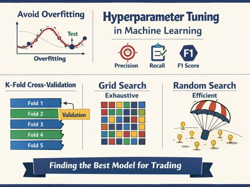
1. The Validation Trap and K-Fold Cross-Validation

If you train a model on your Training Set and tweak the hyperparameters over and over until you get a great score on your Test Set, you have leaked data. Your model hasn’t learned the market; you have just manually optimized it to memorize the Test Set.

To fix this, we use K-Fold Cross-Validation:

• We split the training data into K equal chunks (folds).
• We train the model on K-1 folds and validate it on the remaining 1 fold.
• We repeat this process K times, rotating the validation fold each time.
• The final performance is the average of all K validations. The Test Set remains entirely unseen until the very end.

2. Grid Search (The Exhaustive Approach)

Grid Search is brute force. You give it lists of hyperparameters (e.g., max_depth = [3, 5, 7], n_estimators = [50, 100, 200]). It calculates every single possible combination, runs Cross-Validation for each, and spits out the absolute best one.

• Pros: Guaranteed to find the best combination within your specified grid.
• Cons: The “Curse of Dimensionality”. If you have 5 hyperparameters, each with 5 options, that’s 5^5 = 3,125 combinations. Multiplied by 5-fold CV, that’s 15,625 model trainings. This can take a long time.

3. Random Search (The Efficient Approach)

Instead of testing every combination, Random Search pulls random combinations from a distribution of hyperparameters for a fixed number of iterations.

• Why it works better: In finance, usually, only one or two hyperparameters actually matter (e.g., learning rate). Grid Search wastes time testing every combination of useless hyperparameters. Random Search explores a wider variety of the important hyperparameters much faster.

Trainer’s Tip: We need to use the “Lost Keys in a Field” analogy. Grid Search divides the field into a 1×1 foot grid and checks every square inch sequentially. It guarantees you find the keys, but it takes forever. Random Search means dropping a parachutist randomly into the field 100 times. Mathematically, the parachutist is highly likely to land close enough to spot the keys in a fraction of the time.

The Hands-On Practice

Let’s tune a Random Forest classifier to predict market direction. We will compare the computational time and results of Grid vs. Random Search.

import numpy as np

import pandas as pd

from sklearn.datasets import make_classification

from sklearn.model_selection import train_test_split, GridSearchCV, RandomizedSearchCV

from sklearn.ensemble import RandomForestClassifier

from sklearn.metrics import classification_report

import time

 

# 1. Simulate Financial Signal Data

X, y = make_classification(n_samples=2000, n_features=10, n_informative=5, random_state=42)

X_train, X_test, y_train, y_test = train_test_split(X, y, test_size=0.2, random_state=42)

 

# 2. Define the Hyperparameter Space

param_grid = {

‘n_estimators’: [50, 100, 200],

‘max_depth’: [None, 5, 10, 15],

‘min_samples_split’: [2, 5, 10],

‘min_samples_leaf’: [1, 2, 4]

}

 

# Base Model

rf = RandomForestClassifier(random_state=42)

 

# — GRID SEARCH —

print(“Starting Grid Search…”)

start_time = time.time()

# cv=5 means 5-fold cross validation. n_jobs=-1 uses all CPU cores.

grid_search = GridSearchCV(estimator=rf, param_grid=param_grid, cv=5, n_jobs=-1, scoring=‘accuracy’)

grid_search.fit(X_train, y_train)

grid_time = time.time() – start_time

 

print(f“Grid Search Time: {grid_time:.2f} seconds”)

print(f“Best Grid Parameters: {grid_search.best_params_}”)

 

# — RANDOM SEARCH —

print(“nStarting Random Search…”)

start_time = time.time()

# n_iter=20 means we only test 20 random combinations out of the possible 108.

random_search = RandomizedSearchCV(estimator=rf, param_distributions=param_grid,

n_iter=20, cv=5, n_jobs=-1, scoring=‘accuracy’, random_state=42)

random_search.fit(X_train, y_train)

random_time = time.time() – start_time

 

print(f“Random Search Time: {random_time:.2f} seconds”)

print(f“Best Random Parameters: {random_search.best_params_}”)

 

# 3. Evaluate the Best Model

best_model = random_search.best_estimator_

y_pred = best_model.predict(X_test)

print(“n— Final Model Performance on Unseen Test Set —“)

print(classification_report(y_test, y_pred))

 

Check Your Work:

1. Time Comparison: You should notice that Random Search was significantly faster but achieved an accuracy score identical to the exhaustive Grid Search.
2. Scoring Metrics: We used scoring=’accuracy’. In an imbalanced dataset (like fraud detection), change this to scoring=’f1′ or scoring=’roc_auc’ so the tuning algorithm optimizes for the correct business objective.

Conclusion

Hyperparameter tuning is the bridge between a good mathematical theory and a functional trading strategy. We have learned that while Grid Search leaves no stone unturned, Random Search is often the more pragmatic choice for complex models. Most importantly, wrapping these searches in Cross-Validation ensures we do not fool ourselves into thinking we have found edge when we have merely overfit to noise.

However, Grid and Random searches are “dumb”; they do not learn from their past attempts. In the final part of this series, we will explore intelligent, heuristic searches like Bayesian Optimization and apply them to a live Crypto Trading Strategy.