Why Python is the Lingua Franca of Modern Finance

• A Rich Ecosystem: Python’s greatest asset is its vast collection of open-source libraries like NumPy, Pandas, and Scikit-learn. These are battle-tested tools that provide pre-built, highly-optimized functions for nearly any quantitative task you can imagine.
• Ease of Learning and Readability: Python’s syntax is clean and intuitive. This allows you, the subject matter expert, to focus on the financial logic, not on wrestling with complex code.
• Massive Community: If you hit a roadblock, chances are someone in the massive global Python community has already solved it. The amount of free resources, tutorials, and support is unparalleled.

Setting Up Your Professional Quant Environment

For our purposes, we won’t just install Python; we’ll install the Anaconda Distribution. This is the industry standard for quantitative analysis because it bundles Python with all the essential libraries and tools we’ll need, simplifying the setup process.

Step 1: Download and Install Anaconda

1. Head over to the Anaconda Distribution official website.
2. Download the installer for your operating system (Windows, macOS, or Linux).
3. Run the installer. It’s a standard installation wizard; I recommend you accept all the default settings.

jupyter notebook

This command will launch a server and open a new tab in your web browser, showing the Jupyter file browser.

Your First “Hello, Quant World!” Script

Let’s test our setup to make sure everything is working correctly.

Step 1: Create a New Notebook

In the Jupyter interface, click the “New” button in the top-right corner and select “Python 3 (ipykernel)”. This will open a new, empty notebook.

Step 2: Write and Run the Code

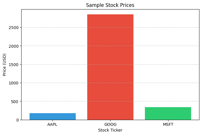
Copy the following code into the first cell of your notebook. This script uses pandas to create a simple portfolio ‘DataFrame’ and matplotlib to plot the data.

import pandas as pd
import matplotlib.pyplot as plt

# Create a sample DataFrame representing a small portfolio
data = {
    'Stock': ['AAPL', 'GOOG', 'MSFT'],
    'Price': [175.30, 2850.50, 340.88]
}
df = pd.DataFrame(data)

# Display the DataFrame
print("My First Portfolio DataFrame:")
print(df)

# Create a simple bar plot of the prices
plt.figure(figsize=(8, 5))
plt.bar(df['Stock'], df['Price'], color=['#3498db', '#e74c3c', '#2ecc71'])
plt.xlabel('Stock Ticker')
plt.ylabel('Price (USD)')
plt.title('Sample Stock Prices')
plt.grid(axis='y', linestyle='--', alpha=0.7)
plt.show()

Step-by-Step Explanation:

1. import pandas as pd: We import the pandas library, giving it the standard alias pd.
2. import matplotlib.pyplot as plt: We import the pyplot module from matplotlib, aliased as plt, for plotting.
3. data = {...}: We create a Python dictionary to hold our sample portfolio data.
4. df = pd.DataFrame(data): We pass our dictionary to the pandas DataFrame constructor to create our main data structure.
5. print(...): We print the DataFrame to the console.
6. plt.figure(...) and plt.bar(...): We use matplotlib to create and customize a bar chart from our data.
7. plt.show(): This command displays the final plot.

To run the code, simply press Shift + Enter while your cursor is in the cell.

Expected Output:

You should see the below text output directly below the cell:

My First Portfolio DataFrame:
  Stock    Price
0  AAPL   175.30
1  GOOG  2850.50
2  MSFT   340.88

And below that, you should see a bar chart:

Conclusion and Next Steps

Congratulations! You’ve successfully set up a professional quantitative analysis environment and run your first script. You now have the foundational tools used across the entire finance industry.

Now that our environment is ready, we need to learn how to represent financial concepts with code. In the next part of this series, we’ll dive into Python’s fundamental data types and control flow, but we’ll do it through the lens of a quant. You’ll learn how a simple number becomes a stock_price, a list becomes a price_history, and an if statement becomes a trading_rule.

Next Up: Part 2: Python’s Building Blocks: A Quant’s Guide to Data Types and Logic