Financial Econometrics: Part 13

Prerequisites: Basics of Stationarity and ACF/PACF

Introduction: From Description to Simulation

In our last article, we established the “rules of the road” for Time Series Analysis. We learned that raw stock prices are often non-stationary (they wander unpredictably) and that we must transform them; usually via Log Returns to create a stationary series that behaves consistently over time.

But once we have a stationary series, what do we do with it?

We need to build a mathematical model that mimics the data’s behavior. If we can write down an equation that generates data looking exactly like our stock returns, we have “solved” the series. We can then use that equation to forecast future risks and opportunities.

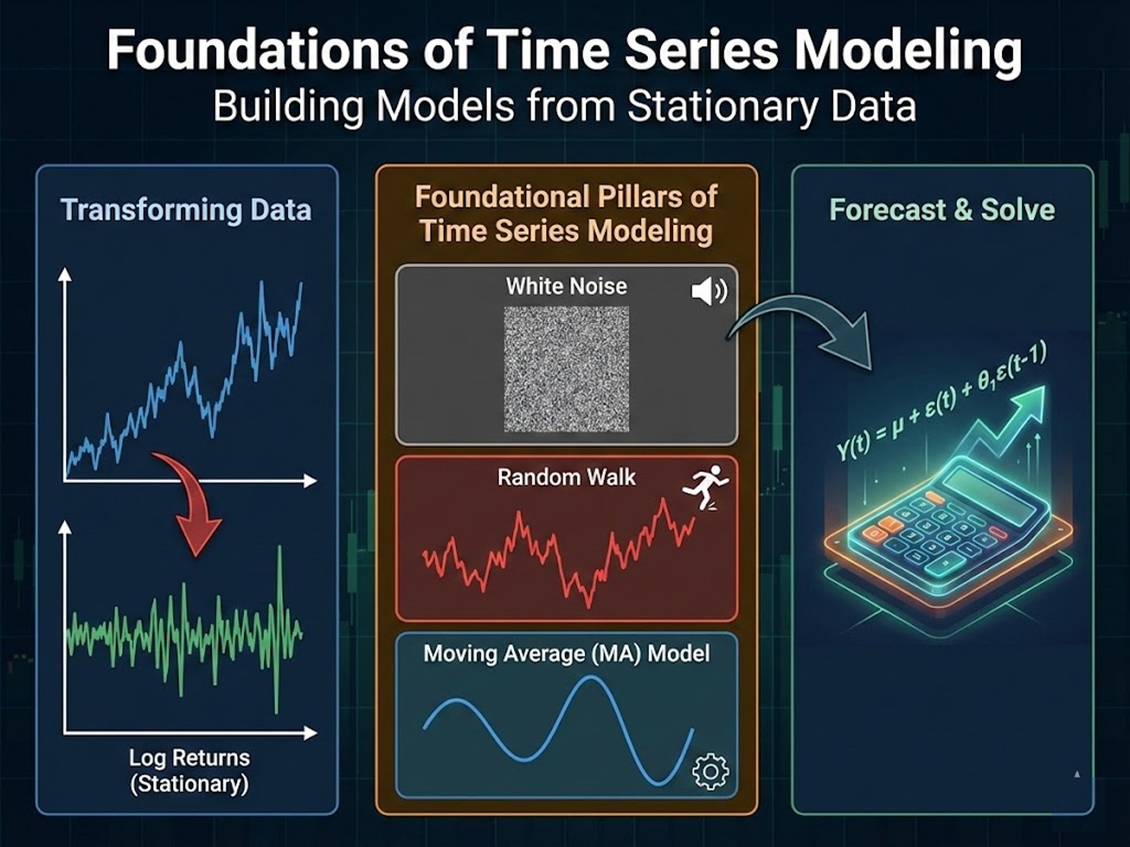
In this article, we will construct the three foundational pillars of time series modeling:

• White Noise: The sound of pure randomness.
• The Random Walk: The “drunkard’s walk” that defines most financial markets.
• The Moving Average (MA) Model: The first model that gives “structure” to the noise.

Part 1: The Sound of Silence (White Noise)

Before we can model patterns, we must define what it looks like when there are no patterns. In Time Series Analysis, this perfect state of randomness is called White Noise.

White Noise is the “blank canvas” of econometrics. It is the ideal error term. When you build a forecasting model (like a regression), your goal is to extract all the signal (trends, seasonality, correlations) until the only thing left in your residuals is White Noise. If your residuals are not White Noise, you have missed something.

The Definition

Note: “i.i.d.” stands for Independent and Identically Distributed.

Why “White”?

The term comes from physics and signal processing. Just as “white light” contains all visible frequencies of light with equal intensity, “white noise” contains a mixture of all frequencies with equal power. It is static. It is the sound of a TV tuned to a dead channel.

Part 2: The Drunkard’s Walk (Random Walk Models)

Now, let’s take our White Noise and do something dangerous with it. Let’s accumulate it.

Imagine a person leaving a bar. They take a step forward. Then, they flip a coin. If it’s heads, they take a step to the left; tails, a step to the right. This is a Random Walk. It is the most fundamental model in finance because it describes (to a frustrating degree) how asset prices move.

The Random Walk with Drift

Stocks generally go up over the long run (due to inflation and economic growth). A pure Random Walk doesn’t capture this; it just wanders aimlessly. To make it realistic, we add a constant $delta$ (delta), known as the Drift.

The Stationarity Trap

Is a Random Walk stationary? No.

Recall from previous article that stationarity requires constant variance. Let’s look at the variance of a Random Walk:

The Fix: Differencing

How do we fix a Random Walk? We use the Difference Operator ($Delta$) we learned in last article.

Part 3: Removing Trends – Two Schools of Thought

When you see a trend in your data, you have two ways to remove it to achieve stationarity. This distinction is subtle but critical for modeling.

Method 1: Deterministic Trend (Regression)

You assume the trend is a perfect, predictable line, like a clock. You model it as:

Method 2: Stochastic Trend (Differencing)

You assume the trend itself is “shifty.” The slope changes; the direction wanders. This is the Random Walk with Drift model.

Here, we don’t fit a straight line. We just look at the changes.

Tip: In finance, always prefer Method 2 (Differencing). Financial trends are rarely deterministic. A recession or a tech boom can change the slope of the trend instantly. Differencing adapts to these structural breaks naturally; regression lines do not.

Part 4: The Ripple Effect – Moving Average (MA) Models

We have White Noise (pure chaos) and Random Walk (accumulated chaos). Now let’s look at our first structured model: the Moving Average (MA) Process.

Warning: Do not confuse this with the “Moving Average” (SMA/EMA) used in technical analysis charts (like the 200-day moving average). They are related mathematically but used very differently.

Properties of MA(1)

Part 5: Practical Lab – Simulating Chaos

We will now use Python to simulate these processes. Understanding simulations is vital—if you know what the “ideal” chart looks like, you can recognize it in real data.

We will simulate White Noise and a Random Walk, and then try to fit an MA model to our Google stock data.

Step 1: Simulating White Noise and Random Walks

import numpy as np
import pandas as pd
import matplotlib.pyplot as plt
import seaborn as sns

sns.set(style="whitegrid")

# Set random seed for reproducibility
np.random.seed(42)

# 1. Simulate White Noise
# 1000 days of random shocks (mean=0, std=1)
white_noise = np.random.normal(loc=0, scale=1, size=1000)

# 2. Simulate Random Walk
# Cumulative sum of white noise
random_walk = np.cumsum(white_noise)

# 3. Simulate Random Walk with Drift
# Add a small constant drift (e.g., 0.1) to every step
drift = 0.1
random_walk_drift = np.cumsum(white_noise + drift)

# Plotting
plt.figure(figsize=(14, 8))

# Plot White Noise
plt.subplot(2, 1, 1)
plt.plot(white_noise, color='cornflowerblue', linewidth=1)
plt.title('White Noise (Stationary)', fontsize=14)
plt.ylabel('Value')

# Plot Random Walks
plt.subplot(2, 1, 2)
plt.plot(random_walk, label='Pure Random Walk', color='gray', linestyle='--')
plt.plot(random_walk_drift, label='Random Walk with Drift (δ=0.1)', color='firebrick')
plt.title('Random Walk vs. Random Walk with Drift (Non-Stationary)', fontsize=14)
plt.ylabel('Value')
plt.legend()

plt.tight_layout()
plt.show()

• Notice how the White Noise stays bound within a horizontal band (like -3 to 3).
• The Random Walk, however, wanders off.
• The “Drift” version looks exactly like a strong Bull Market chart.

Step 2: Fitting an MA Model to Google Data

Now we return to our real-world dataset (data2.csv). In last article, we saw that Google’s Log Returns looked stationary. Let’s see if an MA(1) model fits them well.

We will use the statsmodels library. Note that in modern Python stats, we often use ARIMA but set the AR and I parts to zero to get an MA model. An MA(1) is effectively ARIMA(0, 0, 1).

import pandas as pd
import numpy as np
from statsmodels.tsa.arima.model import ARIMA
import warnings

# Suppress warnings for cleaner output
warnings.filterwarnings("ignore")

# Load Data (Assuming data2.csv is in the working directory)
df = pd.read_csv('data2.csv')
df['Date'] = pd.to_datetime(df['Date'])
df.set_index('Date', inplace=True)

# Calculate Log Returns
df['Log_Ret'] = np.log(df['GOOGLE']).diff().dropna()

# --- Fitting an MA(1) Model ---
# Order = (p, d, q)
# p = 0 (AutoRegressive part - we will cover this next article)
# d = 0 (Integration/Differencing - we already differenced manually via log returns)
# q = 1 (Moving Average part)

model_ma1 = ARIMA(df['Log_Ret'], order=(0, 0, 1))
results_ma1 = model_ma1.fit()

# Display the summary of the model
print(results_ma1.summary()

Analysis of Output:

Look for the ‘ma.L1’ coefficient in the summary table.

Interpretation of the Results

When you run the code, you find that the MA(1) coefficient for Google returns is small or even insignificant. This is common for large-cap stocks! According to the Efficient Market Hypothesis, past shocks should be absorbed instantly, leaving no “hangover” for tomorrow.

If the MA term is significant, it implies market inefficiency; information is taking time to process, or there is overreaction/underreaction occurring in the market.

Conclusion

We have now moved from static descriptions to dynamic processes.

• White Noise gave us a target for our residuals.
• Random Walks explained why prices drift and why uncertainty grows with time.
• MA Models gave us a way to model the persistence of external shocks.

However, the MA model has a limitation: it assumes the current value depends only on errors (shocks). But what if the current value depends on the previous value itself? What if high prices today lead to high prices tomorrow not because of a shock, but because of momentum?

For that, we need the Autoregressive (AR) model. That will be the subject of our next article, where we will finally combine AR and MA to create the legendary ARIMA model.

Stay tuned.