Financial Econometrics: Part 14

Prerequisites: Stationarity, White Noise, MA Models

Introduction: Momentum vs. Shock

In our previous article, we explored the Moving Average (MA) model. The MA model is like a “hangover”; it describes how an external shock (like a surprise earnings report) lingers in the system for a few days before fading away. It is a model of external forces.

But markets are not just driven by news. They are also driven by psychology, momentum, and behavior. If a stock goes up today, it often attracts buyers who push it up tomorrow simply because it went up today. This internal “memory” is not a shock; it is the process feeding on itself.

To model this, we need the Autoregressive (AR) model. And once we have both AR (internal momentum) and MA (external shocks), we can combine them into the most popular time series forecasting tool in history: ARIMA.

Part 1: The Echo of the Past – Autoregressive (AR) Models

An Autoregressive model posits that the current value of a series ($Y_t$) is a weighted sum of its past values, plus a fresh random shock.

The AR(1) Model

The simplest version is the First-Order Autoregressive Process, AR(1):

\(Y_t = \phi_0 + phi_1 Y_{t-1} + \epsilon_t\)

• \(\phi_0\): The intercept (related to the mean).
• \(\phi_1\): The autoregressive coefficient. This is the “memory” parameter.
• \(\epsilon_t\): The White Noise shock.

The Stability Condition:

For an AR(1) model to be stationary (stable), we generally require \(|\phi_1| < 1\).

• If \(\phi_1 = 1\), we have a Random Walk (non-stationary).
• If \(\phi_1 > 1\), the series is Explosive (it grows exponentially to infinity).
• If \(\phi_1 = 0\), the series is just White Noise (no memory).

The AR(p) Model

We can extend this to look back $p$ days. An AR(p) model is:

$$Y_t = \phi_0 + \phi_1 Y_{t-1} + \phi_2 Y_{t-2} + \dots + \phi_p Y_{t-p} + \epsilon_t$$

Visual Diagnostics: AR vs. MA

How do you distinguish an AR process from an MA process just by looking at the plots? We use the ACF and PACF.

Why the difference?

1. In an AR(1) process, today (t) is related to yesterday (t-1), which is related to the day before (t-2). So, t is indirectly related to t-2. The correlation “bleeds” through time, causing the ACF to decay slowly.
2. The PACF removes the intermediate steps. It asks: “Is t related to t-2 after accounting for t-1?” In a pure AR(1) process, the answer is No. The link is purely via t-1. Thus, the PACF spikes at lag 1 and then cuts to zero.

Part 2: The Grand Unification – ARMA and ARIMA

In the real world, data rarely behaves like a pure AR or a pure MA process. It usually has elements of both:

• Momentum (AR): High prices attract buyers.
• Shocks (MA): Bad news causes volatility that lingers.

The ARMA(p, q) Model

We combine them into the Autoregressive Moving Average model:

$$Y_t = \underbrace{\phi_1 Y_{t-1} + \dots + \phi_p Y_{t-p}}_{\text{AR Part}} + \underbrace{\epsilon_t + \theta_1 \epsilon_{t-1} + \dots + \theta_q \epsilon_{t-q}}_{\text{MA Part}}$$

The ARIMA(p, d, q) Model

There is one missing piece: Stationarity. ARMA models only work on stationary data. If your stock price is trending (Random Walk), you cannot use ARMA directly.

You must Difference the data first.

• If you difference the data d times to make it stationary, you are building an ARIMA model.
• I stands for Integrated.

The Three Parameters:

• p (Autoregression): The number of lag observations included in the model (lag order).
• d (Integrated): The number of times the raw observations are differenced (degree of differencing).
• q (Moving Average): The size of the moving average window (order of moving average).

Part 3: The Box-Jenkins Methodology (The Workflow)

Building an ARIMA model is not just about running code; it is an art form known as the Box-Jenkins Method. It follows a strict iterative cycle:

Phase 1: Identification

• Visual Inspection: Does the plot look stationary? If not, increment d (take the first difference).
• Stationarity Test: Use the Augmented Dickey-Fuller (ADF) test. If p-value > 0.05, differencing is needed.
• ACF/PACF Analysis: Once stationary, look at the plots to guess $p$ and $q$.
  • PACF spike at 2 \(\rightarrow\) Try AR(2).
  • ACF spike at 3 \(\rightarrow\) Try MA(3).

Phase 2: Estimation & Selection

• Fit the model using Maximum Likelihood Estimation (MLE).
• The Principle of Parsimony: We want the simplest model that explains the data. A model with 10 parameters will always fit better than a model with 2, but it will overfit (predict noise).
• Information Criteria (AIC & BIC): These are scores that penalize complexity.
  • AIC (Akaike Information Criterion): Good for prediction.
  • BIC (Bayesian Information Criterion): Stricter penalty; good for finding the “true” model.
  • Rule: Lower is Better.

Phase 3: Diagnostic Checking

• Residual Analysis: The residuals of your model must be White Noise.
• Ljung-Box Test: This is a formal statistical test for white noise.
  • \(H_0\): The residuals are independently distributed (White Noise).
  • \(H_a\): The residuals are not independent (Structure remains).
  • Goal: We want a High P-Value (> 0.05) so we fail to reject the null hypothesis.

Part 4: Practical Lab – Python Implementation

Let’s apply the Box-Jenkins methodology to our Google stock data (data2.csv). We will build an ARIMA model to predict returns.

Step 1: Identification (Stationarity Check)

import pandas as pd
import numpy as np
import matplotlib.pyplot as plt
from statsmodels.tsa.stattools import adfuller
from statsmodels.graphics.tsaplots import plot_acf, plot_pacf
import seaborn as sns

sns.set(style="whitegrid")

# Load Data
df = pd.read_csv('data2.csv')
df['Date'] = pd.to_datetime(df['Date'])
df.set_index('Date', inplace=True)

# Create Log Returns (Method 2: Stochastic Trend Removal)
df['Log_Ret'] = np.log(df['GOOGLE']).diff()

# Ensure no NaN or Inf values before ADF test
log_ret_cleaned = df['Log_Ret'].replace([np.inf, -np.inf], np.nan).dropna()

# 1. Augmented Dickey-Fuller Test
# H0: The series is Non-Stationary (has a unit root)
# Ha: The series is Stationary
result = adfuller(log_ret_cleaned)
print(f'ADF Statistic: {result[0]}')
print(f'p-value: {result[1]}')

# Trainer's Interpretation:
# If p-value < 0.05, we confirm the returns are Stationary.
# Therefore, d=0 (for the returns series) or d=1 (for the original price series).

# 2. ACF and PACF Plots to guess p and q
fig, (ax1, ax2) = plt.subplots(2, 1, figsize=(12, 10))
plot_acf(log_ret_cleaned, lags=30, ax=ax1, title='ACF of Log Returns')
plot_pacf(log_ret_cleaned, lags=30, ax=ax2, title='PACF of Log Returns')
plt.tight_layout()
plt.show()

Interpretation:

• If p-value < 0.05, we confirm the returns are Stationary.
• Therefore, d=0 (for the returns series) or d=1 (for the original price series).

Step 2: Estimation (Finding Best p, d, q)

Usually, ACF/PACF plots are messy for real financial data. Instead of guessing, we often perform a “Grid Search” to find the parameters that minimize the AIC.

from statsmodels.tsa.arima.model import ARIMA
import warnings
 
warnings.filterwarnings("ignore")
 
# Define the p, d, q ranges to test
p_values = range(0, 3)
d_values = [0] # We are using returns, so d=0
q_values = range(0, 3)
 
best_aic = float("inf")
best_order = None
best_model = None
 
print("Performing Grid Search...")
for p in p_values:
    for d in d_values:
        for q in q_values:
            try:
                # Fit the model
                model = ARIMA(df['Log_Ret'], order=(p, d, q))
                results = model.fit()
                
                # Compare AIC
                if results.aic < best_aic:
                    best_aic = results.aic
                    best_order = (p, d, q)
                    best_model = results
                
                print(f"ARIMA{p,d,q} - AIC:{results.aic:.2f}")
            except:
                continue
 
print(f"\nBest Model: ARIMA{best_order} with AIC: {best_aic:.2f}")
 
# Print Summary of Best Model
print(best_model.summary())

Step 3: Diagnostics (Ljung-Box Test)

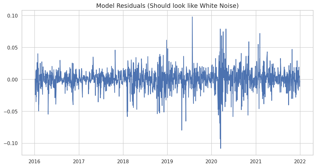
Did we succeed? If the model is good, the residuals should be boring (White Noise).

from statsmodels.stats.diagnostic import acorr_ljungbox

# 1. Visual Check of Residuals
residuals = best_model.resid

plt.figure(figsize=(12, 6))
plt.plot(residuals)
plt.title('Model Residuals (Should look like White Noise)', fontsize=14)
plt.show()

# 2. Ljung-Box Test
# We test up to lag 10
lb_test = acorr_ljungbox(residuals.dropna(), lags=[10], return_df=True) # Drop NaN values from residuals
print("\nLjung-Box Test Results:")
print(lb_test)

Output:

Ljung–Box Test Results:

lb_stat lb_pvalue

1052.248292 1.026474e-07

Interpretation:

Look at the ‘lb_pvalue’.

• If p-value > 0.05: SUCCESS. We accept H0 (Residuals are White Noise). The model is valid.
• If p-value < 0.05: FAILURE. Residuals still have patterns. We need a better model (maybe increase p or q).

Conclusion

We have now reached the summit of classical time series analysis. You understand that:

• AR captures the internal momentum of a market.
• MA captures the lingering effects of external shocks.
• I (Integration) handles the drifting trends.
• ARIMA combines them all into a single, powerful equation.

But there is a catch.

Look closely at the residuals in your plot. You might notice that while the mean is zero, the width of the wiggle changes. Sometimes the market is calm; sometimes it is wild. This “clustering of volatility” violates the constant variance assumption of ARIMA.

ARIMA predicts the mean of the price, but it cannot predict the risk. To model the changing risk (volatility), we need the Nobel Prize-winning ARCH and GARCH models.

That is the topic of our next, and perhaps most exciting article.