Unlocking Market Volatility: A Deep Dive into the ARCH Model

Focus: Volatility Clustering, Heteroskedasticity, and the ARCH(1) Process

Introduction: The Pulse of the Market

If you have ever watched a stock chart during a crisis, you know that panic is contagious. Large market moves rarely happen in isolation. A 3% drop today often increases the probability of a wild swing tomorrow – maybe up, maybe down, but definitely volatile. Conversely, during quiet summers, the market can drift peacefully for weeks with barely a ripple.

This phenomenon is known in finance as Volatility Clustering: large changes tend to be followed by large changes, and small changes by small changes.

As a trainer in financial data science, I often see students try to fit standard linear models (like ARIMA) to financial time series. They often run into a wall. Why? Because standard models assume Homoskedasticity; the fancy statistical word for “constant variance.” They assume the “noise” or “risk” in the market is the same today as it was during the 2008 crash. Intuitively, we know that’s wrong.

In this article of our series, we are going to fix that. We will step away from constant variance and introduce the ARCH (AutoRegressive Conditional Heteroskedasticity) model. We will break down the math step-by-step, explain the intuition, and run Python code to see it in action.

Section 1: The Problem with Constant Variance

Before we build the solution, let’s understand the problem using real data. We will look at Google’s stock price (from the data.csv file).

1.1 Visualizing Returns

When we model asset prices, we usually work with log returns rather than raw prices, as returns are more likely to be stationary.

$$r_t = ln(P_t) – ln(P_{t-1})$$

import pandas as pd
import numpy as np
import matplotlib.pyplot as plt
 
# Load the data
data = pd.read_csv('data.csv')
data['Date'] = pd.to_datetime(data['Date'])
data.set_index('Date', inplace=True)
 
# Calculate Log Returns
data['log_ret'] = np.log(data['GOOGLE']) - np.log(data['GOOGLE'].shift(1))
 
# Plotting
plt.figure(figsize=(12, 6))
plt.plot(data['log_ret'])
plt.title('Google Daily Log Returns')
plt.ylabel('Log Return')
plt.xlabel('Date')
plt.grid(True)
plt.show()

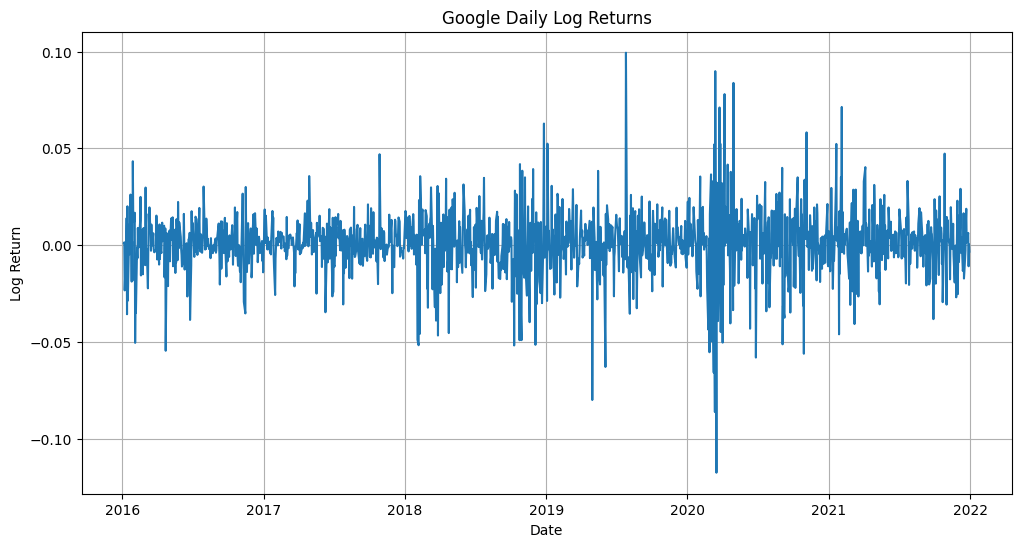
What do we see?

If the variance were constant, this plot would look like a uniform band of noise with the same width from left to right. Instead, we see “bursts” of activity. There are periods where the noise spikes (high volatility) and periods where it is flat (low volatility).

This visual evidence confirms Conditional Heteroskedasticity. The variance conditional on the past is changing.

Section 2: Enter the ARCH Model

In 1982, Robert Engle introduced the ARCH model to capture this behavior (winning a Nobel Prize for it later). The core idea is simple but powerful: The variance of tomorrow depends on the square of the shock today.

2.1 The Two Equations of ARCH(1)

An ARCH model consists of two distinct parts:

• The Mean Equation: Describes the average behavior of the series (often just zero or a constant).
• The Variance Equation: Describes how the variance changes over time.

Let’s look at the ARCH(1) model, the simplest form.

The Mean Equation

The Variance Equation

Let’s decode this:

Section 3: Deep Dive into Properties

To really understand ARCH, we need to look at its statistical properties. This is often where learners get lost, so let’s take it step-by-step.

3.1 Unconditional Mean

$$ E[a_t] = 0 $$

Takeaway: The ARCH model doesn’t predict direction (up or down); it predicts magnitude (risk).

3.2 Unconditional Variance

So, the equation becomes:

3.3 Fat Tails (Kurtosis)

Section 4: Simulating ARCH in Python

import numpy as np
import matplotlib.pyplot as plt
 
# 1. Set Parameters
n = 1000  # number of data points
alpha0 = 1
alpha1 = 0.5
 
# 2. Initialize arrays
a = np.zeros(n)      # returns
sigma2 = np.zeros(n) # variances
 
# 3. Simulation Loop
# We need a starting value. Let's assume a[0] = 0 for simplicity.
np.random.seed(42)
 
for t in range(1, n):
    # Calculate current variance based on previous squared return
    sigma2[t] = alpha0 + alpha1 * (a[t-1]**2)
    
    # Calculate current return: std_dev * random_shock
    a[t] = np.sqrt(sigma2[t]) * np.random.normal(0, 1)
 
# 4. Plotting
plt.figure(figsize=(12, 8))
 
# Plot Returns
plt.subplot(2, 1, 1)
plt.plot(a)
plt.title(f'Simulated ARCH(1) Returns (alpha0={alpha0}, alpha1={alpha1})')
plt.ylabel('Return (a_t)')
 
# Plot Conditional Variance
plt.subplot(2, 1, 2)
plt.plot(sigma2, color='orange')
plt.title('Conditional Variance (sigma^2_t)')
plt.ylabel('Variance')
plt.xlabel('Time')
 
plt.tight_layout()
plt.show()

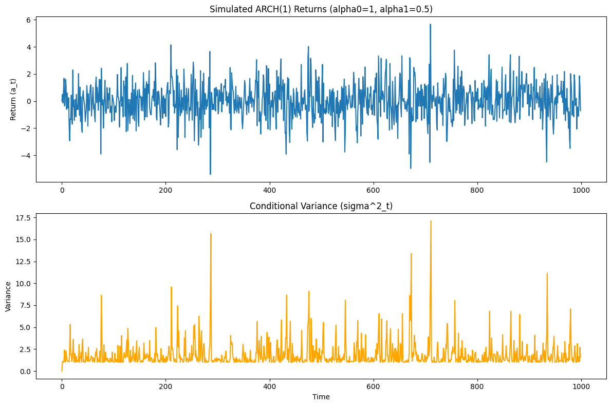
Observation

When you run this code, look at the two plots.

1. Simulated ARCH(1) Returns: You will see “bursts” of noise.
2. Conditional Variance: You will see the variance spiking exactly when the returns are large.

This confirms that our mathematical model successfully generates volatility clustering!

Section 5: The ARCH(m) Model

Weaknesses of ARCH(m)

While ARCH(m) is better, it has practical issues:

This limitation sets the stage for the GARCH model (Generalized ARCH), which solves the “too many parameters” problem.

Conclusion & Next Steps

In this article, we moved from the naive assumption of constant variance to the dynamic world of Conditional Heteroskedasticity.

Key Takeaways:

However, as we noted, pure ARCH models can be cumbersome if we need to look far into the past. In next part, we will introduce the industry-standard GARCH Model. We will see how it achieves “infinite memory” with just a few parameters and apply it to our Google dataset to calculate real-world risk metrics.

Stay tuned!