Taming the Volatility Beast: The GARCH Model

Keywords: GARCH(1,1), Maximum Likelihood Estimation, and Model Diagnostics

Introduction: The Memory of Markets

In last article, we discovered that financial markets are not random walks with constant risk. They are moody. They have “bursts” of panic and periods of calm. We modeled this using ARCH (AutoRegressive Conditional Heteroskedasticity), where today’s volatility depends on yesterday’s shock.

But we hit a wall. To capture the long memory of a market (e.g., the lingering fear after a major crash), an ARCH model needs to look back many days. An ARCH(20) model requires estimating 20 separate parameters. In statistics, this is a nightmare. The more parameters you estimate, the more uncertainty you introduce, and the more likely you are to violate mathematical constraints (like variance becoming negative).

Enter the GARCH (Generalized ARCH) model.

Proposed by Tim Bollerslev in 1986, GARCH is to volatility what ARMA is to price. It solves the parameter explosion problem elegantly. Instead of needing 20 parameters to remember the past, GARCH needs just three.

In this session, we will upgrade our toolkit from ARCH to GARCH. We will define the math, explore its “persistence” property, fit a model to our Google stock data using Python, and, crucially, learn how to check if our model is actually working.

Section 1: The GARCH(1,1) Revolution

The genius of GARCH is a simple recursive trick.

In a GARCH(m, s) model, variance depends on past squared shocks AND past variances.

Let’s focus on the industry standard: GARCH(1,1).

1.1 The Equations

Just like ARCH, we have two equations:

1.2 Why is this better than ARCH?

Section 2: Properties of GARCH

Instead, we use Maximum Likelihood Estimation (MLE).

3.1 The Intuition of MLE

Section 4: Python Implementation

Let’s apply this to our Google data. We will use the arch library, which is the standard Python package for this work.

4.1 Setup and Fitting

We will fit a GARCH(1,1) model to the Google Log Returns.

import pandas as pd

import numpy as np

from arch import arch_model

import matplotlib.pyplot as plt

 

# 1. Load and Prepare Data

data = pd.read_csv(‘data.csv’)

data[‘Date’] = pd.to_datetime(data[‘Date’])

data.set_index(‘Date’, inplace=True)

data[‘log_ret‘] = 100 * (np.log(data[‘GOOGLE’]) – np.log(data[‘GOOGLE’].shift(1)))

data.dropna(inplace=True)

 

# Note: We multiply by 100 to convert to percentages.

# GARCH optimizers work better when data is scaled to be > 1.

 

# 2. Define the Model

# vol=’Garch‘: Specifies the variance model

# p=1, q=1: The lag orders (GARCH(1,1))

# mean=’Zero’: We assume mean return is approx zero for simplicity

model = arch_model(data[‘log_ret‘], vol=‘Garch‘, p=1, q=1, mean=‘Zero’)

 

# 3. Fit the Model

res = model.fit(disp=‘off’)

 

# 4. Print Summary

print(res.summary())

 

4.2 Interpreting the Output

When you run the code above, you will get a summary table. Here is how to read it:

• $omega$ (const): The baseline variance.
• $alpha$ (alpha[1]): Reaction to news.
• $beta$ (beta[1]): Persistence.

Result Check:

1. The Persistence Check ($beta approx 0.9$)

Look at the coefficient for beta[1]. In daily financial data, this is almost always between 0.85 and 0.98.

1. What it means: High persistence. If a major news event spikes volatility today, it won’t vanish tomorrow. It will decay slowly over weeks.
2. Red Flag: If $beta$ is small (e.g., 0.1), your model might be failing to capture the trend, or the asset truly has no memory (rare).

2. The Stationarity Check ($alpha + beta < 1$)

Add the alpha[1] and beta[1] coefficients together.

• The Rule: The sum must be less than 1.
• Why? If the sum is $ge 1$, the long-run variance ($V_L$) becomes undefined (dividing by zero or negative). This is called an IGARCH (Integrated GARCH) process, implying volatility drifts forever and never returns to a normal level.
• Common Scenario: For stocks, a sum of 0.95-0.99 is common. This indicates “very slow” mean reversion.

3. The Significance Check (P-values)

Check the P>|t| column.

• The Rule: We generally want p-values $< 0.05$.
• Analysis:
  • If $alpha$ is not significant: Recent news doesn’t impact volatility much.
  • If $beta$ is not significant: Volatility has no memory.
  • If $omega$ is not significant: This is sometimes acceptable, but implies the baseline variance is near zero.

4. Google Data

The model is stable (0.95 < 1). It is highly persistent (0.95 is close to 1), meaning the current volatile period will likely last for some time.

4.3 Visualizing the Volatility

The res object contains the estimated conditional volatility. Let’s plot it.

# Plotting the estimated volatility

fig = res.plot(annualize=‘D’)

plt.show()

 

# Extracting the conditional volatility

data[‘volatility’] = res.conditional_volatility

plt.figure(figsize=(10,6))

plt.plot(data[‘log_ret‘], color=‘grey’, alpha=0.5, label=‘Returns’)

plt.plot(data[‘volatility’], color=‘red’, label=‘GARCH Volatility’)

plt.title(‘Google Returns vs GARCH Volatility’)

plt.legend()

plt.show()

 

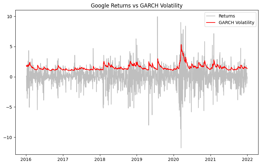
The red line tracks the risk. Notice how it spikes during the turbulent periods and calms down after them. This is exactly what we wanted: a dynamic risk metric.

Section 5: Model Diagnostics (The “Sanity Check”)

A common mistake in data science is fitting a model and walking away. We must check if the model is valid.

If the GARCH model has done its job, it should have “explained away” all the volatility clustering. The leftovers, called Standardized Residuals, should look like boring, random white noise.

$$ Z_t = frac{a_t}{sigma_t} $$

If $Z_t$ still shows clustering, our model failed (maybe we need GARCH(2,2) or a Student-t distribution).

5.1 The Ljung-Box Test

We check for autocorrelation in the squared standardized residuals.

from statsmodels.stats.diagnostic import acorr_ljungbox

 

# Calculate Standardized Residuals

std_resid = res.resid / res.conditional_volatility

 

# Perform Ljung-Box test on Squared Standardized Residuals

lb_test = acorr_ljungbox(std_resid**2, lags=[10], return_df=True)

print(“Ljung-Box Test on Squared Residuals:”)

print(lb_test)

 

Interpretation:

• Null Hypothesis: No autocorrelation (Good).
• Alternative Hypothesis: Autocorrelation exists (Bad).
• If p-value > 0.05, we fail to reject the null. This is what we want! It means there is no “leftover” volatility pattern. The model has captured it all.

5.2 Normality Test

Standard GARCH assumes errors are Normal. Let’s check.

from scipy.stats import jarque_bera

 

jb_test = jarque_bera(std_resid)

print(f“Jarque-Bera p-value: {jb_test.pvalue}”)

 

In finance, this test often fails (p < 0.05) because returns have “fat tails” even after GARCH filtering. This suggests we might need to use a Student-t distribution for the error term in the GARCH model (an option dist=’t’ in the arch_model function).

Section 6: GARCH(p,q) and Beyond

While GARCH(1,1) is the workhorse, the general form is GARCH(p,q):

$$ sigma_t^2 = omega + sum_{i=1}^{q} alpha_i a_{t-i}^2 + sum_{j=1}^{p} beta_j sigma_{t-j}^2 $$

• $q$: Number of lag shocks (ARCH terms).
• $p$: Number of lag variances (GARCH terms).

Increasing $p$ and $q$ adds complexity. Usually, $p=1, q=1$ is sufficient. If you need higher orders, it’s often a sign that the underlying process is more complex than a simple GARCH can handle, or that there are “structural breaks” (e.g., a permanent shift in market regulation) that you are ignoring.

Conclusion

We have successfully tamed the volatility beast.

• GARCH(1,1) allows us to model “infinite memory” volatility with just 3 parameters.
• Mean Reversion: We can calculate the long-run average risk.
• Diagnostics: We learned that a good model leaves behind “clean” white noise residuals.

However, we relied entirely on Maximum Likelihood Estimation (MLE). MLE gives us a single “best guess” for $alpha$ and $beta$. But what if the data is scarce? What if we have prior beliefs about market behavior?

In next article, we will leave the frequentist world behind and enter the Bayesian universe. We will learn how to estimate GARCH models using MCMC (Markov Chain Monte Carlo), allowing us to quantify the uncertainty of our parameters themselves.

Get your priors ready!