Building a Time Series Momentum Strategy with Linear Regression

Introduction

For quantitative analysts, moving from heuristic-based trading rules to data-driven Machine Learning (ML) models is a critical evolution. While traditional statistical arbitrage relies on pre-defined correlations, Machine Learning allows us to uncover complex, non-linear patterns in historical data.

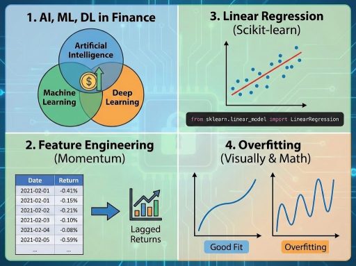
In this first instalment of our Machine Learning for Quants series, we will demystify the foundations of Supervised Learning. We won’t just talk theory; we will build a working Time Series Momentum strategy using Linear Regression to predict S&P 500 (SPY) returns. We will also demonstrate the critical concept of “overfitting”; the most common pitfall in financial ML.

Learning Objectives

By the end of this tutorial, you will be able to:

1. Differentiate between Artificial Intelligence (AI), Machine Learning (ML), and Deep Learning (DL) in a financial context.
2. Engineer features for a Momentum strategy by creating lagged return datasets.
3. Train and evaluate a Linear Regression model using scikit-learn.
4. Identify overfitting visually and mathematically when model complexity exceeds signal availability.

Prerequisites

To follow this tutorial, you will need:

1. Python 3.7+ installed.
2. Jupyter Notebook or a similar IDE (VS Code, Google Colab).
3. Financial Data Access: An active internet connection to download market data via yfinance.
4. Required Libraries:
   1. numpy
   2. pandas
   3. matplotlib
   4. scikit-learn
   5. yfinance

Core Concepts (The Theory)

1. The ML Hierarchy: AI vs. ML vs. DL

It is crucial to understand where our work fits:

• Artificial Intelligence (AI): The broad effort to automate intellectual tasks. A rule-based algo (“Buy if MA50 > MA200”) is AI, but not ML.
• Machine Learning (ML): A subset of AI where the system learns rules from data rather than having them explicitly programmed. We feed it input (past returns) and output (future returns), and it figures out the relationship.
• Deep Learning (DL): A subset of ML using multi-layered neural networks to learn representations.

2. Supervised Learning & Linear Regression

We are performing Supervised Learning because we have a labelled dataset: we know the actual past returns (labels) associated with our historical indicators (features).

We will use Linear Regression, the “Hello World” of quantitative ML. It attempts to model the relationship between a dependent variable $y$ (future return) and independent variables $X$ (past returns) using a linear equation:

$$ hat{y} = theta_0 + theta_1 x_1 + theta_2 x_2 + dots + theta_n x_n $$

Where:

• $hat{y}$ is the predicted value.
• $x_i$ are the features (e.g., return yesterday, return 2 days ago).
• $theta$ (theta) are the parameters (weights) the model “learns” during training to minimize error.

3. The Overfitting Trap

In finance, data is noisy. Overfitting occurs when a model learns the “noise” (random market fluctuations) rather than the “signal” (actual trends).

• Underfitting: The model is too simple (e.g., a straight line trying to fit a curve).
• Overfitting: The model is too complex (e.g., a high-degree polynomial connecting every single dot). It looks perfect on past data but fails miserably on new, unseen data.

Step-by-Step Walkthrough (The Hands-On Practice)

Step 1: Setup and Data Acquisition

First, we will import our tools and fetch historical data for the SPY ETF (S&P 500).

import numpy as np

import pandas as pd

import yfinance as yf

import matplotlib.pyplot as plt

from sklearn.linear_model import LinearRegression

from sklearn.metrics import mean_squared_error

from sklearn.model_selection import train_test_split

from sklearn.preprocessing import PolynomialFeatures

 

# Download historical data for SPY

# We use a long window to ensure enough data points

df = yf.download(‘SPY’, start=‘2013-01-01′, end=‘2026-01-01′)

 

# Calculate daily returns

df[‘Return’] = df[‘Close’].pct_change()

 

# Drop NaN values created by pct_change

df.dropna(inplace=True)

 

print(f“Data Loaded: {len(df)} days of trading data.”)

print(df.head())

 

Step 2: Feature Engineering (The Momentum Signal)

A Momentum strategy relies on the idea that past performance influences future results. We will create “lagged” features; using returns from $t-1$, $t-2$, etc., to predict the return at time $t$.

# Create lag features (signals)

# We want to use the returns of the past 5 days to predict today’s return

lags = 5

 

for i in range(1, lags + 1):

df[f‘Lag_{i}’] = df[‘Return’].shift(i)

 

# Drop the NaN values created by shifting

df.dropna(inplace=True)

 

# Define Features (X) and Target (y)

feature_cols = [f‘Lag_{i}’ for i in range(1, lags + 1)]

X = df[feature_cols]

y = df[‘Return’]

 

print(“Feature Matrix X (First 5 rows):”)

print(X.head())

 

Step 3: Splitting the Dataset

We must never evaluate a model on the same data used to train it. In time-series finance, we cannot shuffle data randomly (because time matters). We split chronologically.

# Split into Training (80%) and Testing (20%) sets

# shuffle=False is CRITICAL for time series data

X_train, X_test, y_train, y_test = train_test_split(X, y, test_size=0.2, shuffle=False)

 

print(f“Training set size: {len(X_train)}”)

print(f“Testing set size: {len(X_test)}”)

 

Step 4: Training the Linear Regression Model

Now, we instantiate the model and fit it to our training data.

# Initialize the model

lr_model = LinearRegression()

 

# Train the model

lr_model.fit(X_train, y_train)

 

# View learned coefficients (The “Theta” values)

print(“Intercept (Bias):”, lr_model.intercept_)

print(“Coefficients (Weights):”, lr_model.coef_)

 

Step 5: Evaluation and Visualizing Performance

Let’s see how well our simple model predicts returns.

# Make predictions on the test set

y_pred = lr_model.predict(X_test)

 

# Calculate Mean Squared Error (MSE)

mse = mean_squared_error(y_test, y_pred)

print(f“Mean Squared Error (Linear Model): {mse:.8f}”)

 

# Visualization: Predicted vs Actual (Subset for clarity)

plt.figure(figsize=(12, 6))

plt.plot(y_test.values[:100], label=‘Actual Returns’, alpha=0.7)

plt.plot(y_pred[:100], label=‘Predicted Returns’, alpha=0.7, linestyle=‘–‘)

plt.title(‘Linear Regression: Actual vs Predicted Returns (First 100 Test Days)’)

plt.legend()

plt.show()

 

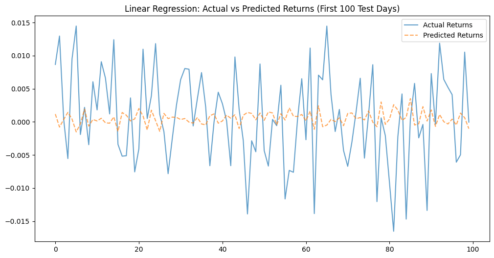
Note: You will notice the predictions are a “flat line” compared to the actual volatility. This is Underfitting. The linear relationship is too weak to capture market noise.

Step 6: Forcing Overfitting (Polynomial Features)

To understand overfitting, let’s intentionally make the model too complex by adding polynomial features (powers of the existing features).

# Create polynomial features (degree 4 – highly complex)

poly = PolynomialFeatures(degree=4)

X_train_poly = poly.fit_transform(X_train)

X_test_poly = poly.transform(X_test)

 

# Train a new model on this complex data

poly_model = LinearRegression()

poly_model.fit(X_train_poly, y_train)

 

# Predict on Train and Test

y_train_pred_poly = poly_model.predict(X_train_poly)

y_test_pred_poly = poly_model.predict(X_test_poly)

 

# Calculate Errors

train_mse = mean_squared_error(y_train, y_train_pred_poly)

test_mse = mean_squared_error(y_test, y_test_pred_poly)

 

print(f“Training MSE (Poly Model): {train_mse:.8f}”)

print(f“Testing MSE (Poly Model): {test_mse:.8f}”)

 

Interpretation: You see that the Training MSE is low (good fit), but the Testing MSE is massive (terrible fit). The model memorized the training data but cannot generalize.

Verification & Independent Practice

Check Your Work

• Shape Check: Ensure X_train has 5 columns (Lag_1 to Lag_5).
• Date Alignment: Check that the index of X_test follows directly after X_train.
• Output Logic: Your Linear Regression coefficients should be small numbers (close to 0), indicating a weak linear signal in efficient markets.

Challenge: The “Window” Hunt

Modify the code in Step 2 to change the lags variable from 5 to 20.

• Does increasing the amount of history (features) improve the Test MSE?
• Does it make the overfitting worse when you apply the Polynomial transformation?

Conclusion & Next Steps

In this tutorial, we established the pipeline for a quantitative machine learning experiment: Data Loading -> Feature Engineering -> Train/Test Split -> Modeling -> Evaluation.

We discovered that a simple Linear Regression tends to underfit financial data (it’s too simple), while high-degree Polynomial Regression overfits (it memorizes noise).

Next Steps:

How do we find the “Goldilocks” zone: a model complex enough to learn but robust enough to generalize? The answer lies in Regularization. In next part, we will cover Ridge, Lasso, and ElasticNet regressions to mathematically penalize complexity and improve our trading strategy.

Troubleshooting / FAQ

Q: My y_pred is almost a straight line at zero.

A: This is expected in financial returns. Daily returns are very close to zero, and the “signal” from past returns is weak. This confirms that simple linear relationships are often insufficient for raw price prediction without more complex features or regularization.

Q: yfinance failed to download data.

A: Ensure you have an active internet connection. Occasionally, the Yahoo Finance API rate-limits requests. Wait a minute and try again, or download a CSV of SPY data manually and load it using pd.read_csv().

Q: Why use shuffle=False in train_test_split?

A: Financial data is sequential. If you shuffle, you might use data from 2022 to predict data from 2015, which is “look-ahead bias”—cheating by knowing the future. Always keep the timeline intact.