
Welcome to the fascinating world of options trading! Think of options as the Swiss Army knife in a financial trader/analyst toolkit. They are incredibly versatile, allowing you to tailor your market position with precision, whether you’re speculating on a big price swing, hedging an existing portfolio, or generating income. But like any powerful tool, you need to understand how to use them safely and effectively.
At their core, options are contracts that give the holder the right, but not the obligation, to buy or sell an underlying asset at a predetermined price within a specific timeframe. The two fundamental types are calls (the right to buy) and puts (the right to sell).
There are sophisticated mathematical models for calculating the precise price of an option, such as the famous Black-Scholes model (an analytical method) or computational approaches like binomial trees (a numerical method). However, before we can run, we must learn to walk. The first step in mastering options is to understand their payoff structure. What happens to your profit or loss as the underlying stock price moves?
In this article, we’ll build that foundational knowledge from the ground up. We will explore:
- The Four Basic Building Blocks: Understanding the unique risk and reward profile of buying and selling calls and puts.
- Visualizing Profit and Loss: Using Python to create payoff diagrams that bring these concepts to life.
- Combining Forces: Graduating to multi-leg strategies like Straddles, Strangles, and Iron Condors to execute on more nuanced market views.
- Practical Application: A step-by-step guide to plotting your own custom strategies.
Let’s open the toolkit and get started.
1. The Building Blocks: Payoffs of Single Options
Every complex option strategy is built from just four basic transactions. A payoff diagram is our most important tool here. It’s a simple graph that plots your potential profit or loss (P&L) at the moment the option expires against a range of possible stock prices.
For our examples, we will use the powerful yet intuitive Python library opstrat, which is designed specifically for plotting and analyzing option strategies.
The Long Call: A Bet on the Upside
When you buy a call option, you are expressing a bullish view. You believe the price of the underlying stock is going to rise significantly.
- How it Works: You pay a premium (the price of the option) for the right to buy a stock at a specific price (the strike price, K).
- Your Goal: For the stock price (S) to rise well above the strike price before the option expires.
- Risk vs. Reward: Your maximum loss is limited to the premium you paid. If the stock price doesn’t rise above the strike, you simply let the option expire worthless. Your potential profit is theoretically unlimited; the higher the stock goes, the more you make.
- Payoff Formula: Profit/Loss = max(0, Stock Price – Strike Price) – Premium Paid
Let’s visualize this with code. Suppose we buy a call option with a strike price of $210 for a premium of $3.25.
import opstrat as op
import matplotlib.pyplot as plt

# Define the parameters for a long call option
long_call = {
    'op_type': 'c',      # 'c' for call
    'st': 210,           # Strike price
    'tr_type': 'b',      # 'b' for buy
    'op_pr': 3.25        # Option premium
}

# Use opstrat to plot the payoff diagram
op.single_plotter(
    spot=210,            # Current stock price
    strike=long_call['st'],
    op_type=long_call['op_type'],
    tr_type=long_call['tr_type'],
    op_pr=long_call['op_pr']
)
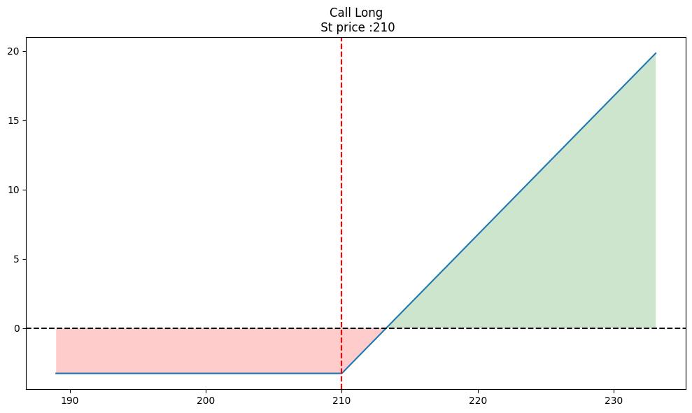
The diagram clearly shows our P&L profile. The horizontal line at -$3.25 represents our maximum loss. The line starts to slope upwards at the strike price of $210. The break-even point, where we start making a profit, is the strike price plus the premium paid: $210 + $3.25 = $213.25.
The Short Call: A Risky Bet on Stagnation
Selling a call option (also known as writing a call) is the other side of the trade. You are expressing a neutral to bearish view.
- How it Works: You receive a premium for giving someone else the right to buy a stock from you at the strike price.
- Your Goal: For the stock price to stay below the strike price.
- Risk vs. Reward: Your maximum profit is limited to the premium you received. However, your potential loss is theoretically unlimited. If the stock price rises; the buyer will exercise their right, forcing you to sell them the stock at a price far below its market value.
- Payoff Formula: Profit/Loss = min(0, Strike Price – Stock Price) + Premium Received
Let’s plot the short version of the same call option.
# Define the parameters for a short call option
short_call = {
    'op_type': 'c',      # 'c' for call
    'st': 210,           # Strike price
    'tr_type': 's',      # 's' for sell
    'op_pr': 3.25        # Option premium
}

# Plot the payoff
op.single_plotter(
    spot=210,
    strike=short_call['st'],
    op_type=short_call['op_type'],
    tr_type=short_call['tr_type'],
    op_pr=short_call['op_pr']
)
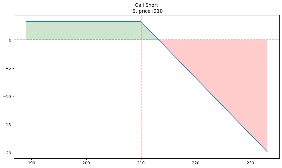
This is a mirror image of the long call. The maximum profit is capped at the premium received ($3.25). The position starts losing money above the break-even point of $213.25, with losses accelerating as the stock price rises.
The Long Put: Profiting from a Decline
If you are bearish and believe a stock’s price will fall, you can buy a put option.
- How it Works: You pay a premium for the right to sell a stock at the strike price.
- Your Goal: For the stock price to fall well below the strike price.
- Risk vs. Reward: Your maximum loss is limited to the premium paid. Your maximum profit is substantial but capped, as a stock’s price cannot fall below zero.
- Payoff Formula: Profit/Loss = max(0, Strike Price – Stock Price) – Premium Paid
Let’s model buying a put with a $210 strike for a $4.50 premium.
# Define the parameters for a long put option
long_put = {
    'op_type': 'p',      # 'p' for put
    'st': 210,           # Strike price
    'tr_type': 'b',      # 'b' for buy
    'op_pr': 4.50        # Option premium
}

# Plot the payoff
op.single_plotter(
    spot=210,
    strike=long_put['st'],
    op_type=long_put['op_type'],
    tr_type=long_put['tr_type'],
    op_pr=long_put['op_pr']
)
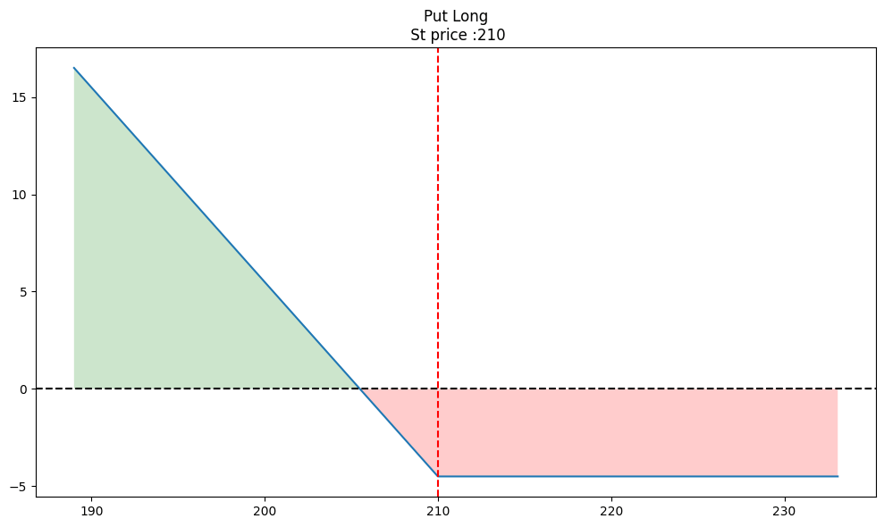
The diagram shows the maximum loss is the premium paid ($4.50). Profits begin to accrue as the stock price falls below the break-even point of $210 – $4.50 = $205.50.
The Short Put: A Bet on Stability or Growth
Selling a put is a neutral to bullish strategy.
- How it Works: You receive a premium for giving someone else the right to sell a stock to you at the strike price.
- Your Goal: For the stock price to stay above the strike price.
- Risk vs. Reward: Your maximum profit is limited to the premium. Your potential loss is substantial, though capped (as the stock can only fall to $0).
- Payoff Formula: Profit/Loss = min(0, Stock Price – Strike Price) + Premium Received
# Define the parameters for a short put option
short_put = {
    'op_type': 'p',      # 'p' for put
    'st': 210,           # Strike price
    'tr_type': 's',      # 's' for sell
    'op_pr': 4.50        # Option premium
}

# Plot the payoff
op.single_plotter(
    spot=210,
    strike=short_put['st'],
    op_type=short_put['op_type'],
    tr_type=short_put['tr_type'],
    op_pr=short_put['op_pr']
)
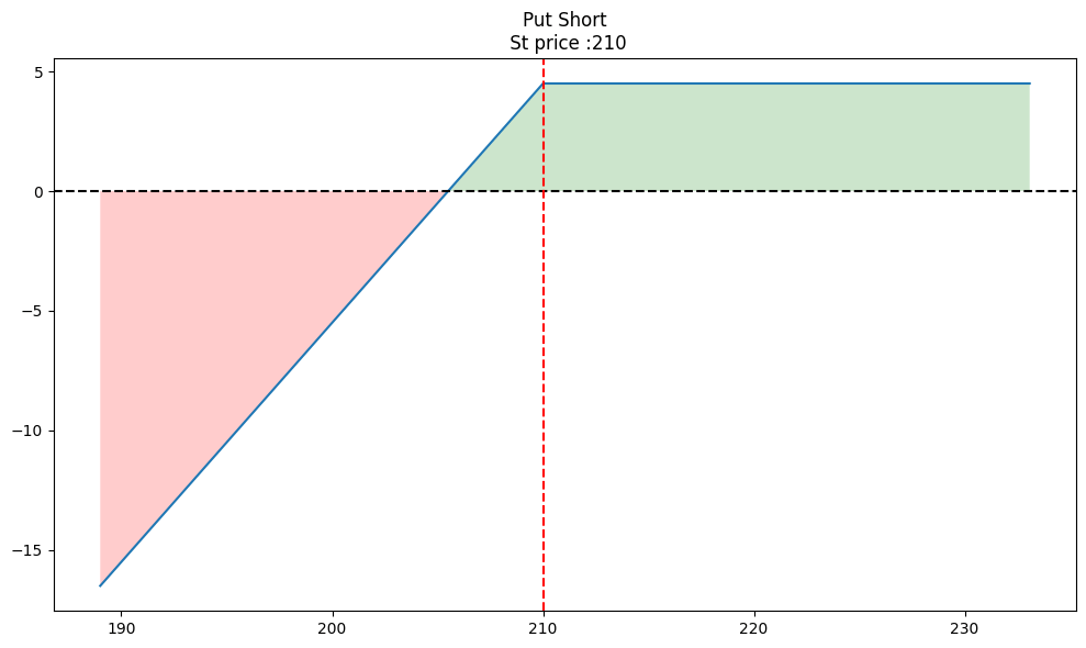
The payoff is capped at the premium received ($4.50). The position becomes unprofitable below the break-even point of $205.50.
2. Combining Forces: Multi-Leg Option Strategies
Now that we understand the building blocks, we can start combining them to create strategies that are more tailored to a specific market forecast.
The Straddle: Betting on a Big Move (in Either Direction)
What if you’re certain a stock is about to make a huge price move, but you have no idea which way it will go? This often happens around major news events like earnings reports or regulatory decisions. The long straddle is the perfect tool for this scenario.
- The Build: Buy one call option and one put option with the same strike price and same expiration date.
- The Logic: If the stock soars, your call option profits. If the stock crashes, your put option profits. You only lose money if the stock price stays relatively stagnant, and your maximum loss is the total premium you paid for both options.
Let’s plot a straddle using our previous examples: buying a $210 call for $3.25 and a $210 put for $4.50.
# Define the two legs of the straddle
straddle_leg1 = {'op_type': 'c', 'strike': 210, 'tr_type': 'b', 'op_pr': 3.25}
straddle_leg2 = {'op_type': 'p', 'strike': 210, 'tr_type': 'b', 'op_pr': 4.50}

# Combine them into a list
option_strategy = [straddle_leg1, straddle_leg2]

# Plot the combined strategy
op.multi_plotter(spot=210, op_list=option_strategy)
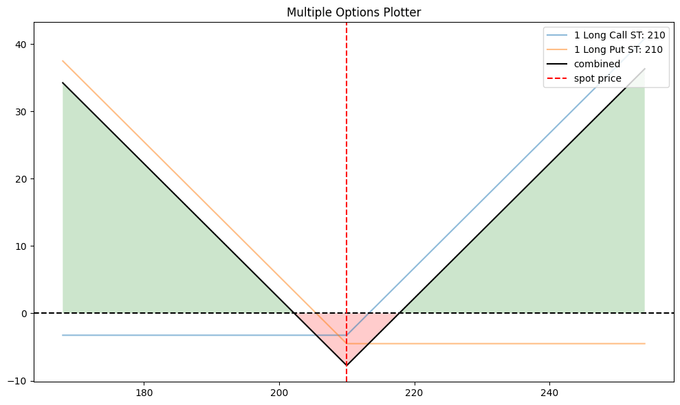
The iconic “V-shape” of the straddle shows that you profit from high volatility. Your maximum loss is $3.25 + $4.50 = $7.75 per share, which occurs only if the stock price finishes exactly at the $210 strike price. There are two break-even points:
- Upside: $210 + $7.75 = $217.75
- Downside: $210 – $7.75 = $202.25
The Strangle: A Cheaper Bet on Volatility
A long strangle is a close cousin of the straddle. It also profits from a large price move in either direction, but it’s constructed with out-of-the-money (OTM) options, making it cheaper to implement.
- The Build: Buy one OTM call option and one OTM put option with the same expiration but different strike prices.
- The Logic: The concept is the same as the straddle, but because the options are OTM, the initial cost (and thus the maximum loss) is lower. The trade-off is that the stock price must move even further before the strategy becomes profitable.
Let’s build a strangle by buying a $220 call and a $200 put.
# Define the two legs of the strangle
strangle_leg1 = {'op_type': 'c', 'strike': 220, 'tr_type': 'b', 'op_pr': 2.50}
strangle_leg2 = {'op_type': 'p', 'strike': 200, 'tr_type': 'b', 'op_pr': 3.00}

option_strategy = [strangle_leg1, strangle_leg2]

op.multi_plotter(spot=210, op_list=option_strategy)
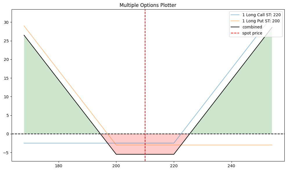
Notice the flat bottom of the “V”. This represents the range between the two strike prices where you incur the maximum loss, which is the total premium paid ($2.50 + $3.00 = $5.50). The stock must move outside this wider range for you to profit.
The Iron Condor: Profiting from Stability
What if your market view is the exact opposite? You believe a stock will be very stable and trade within a narrow price range for the foreseeable future. For this, you can use an iron condor. It’s a more complex, four-legged strategy designed to profit from low volatility.
- The Build:
- Sell an OTM put.
- Buy a further OTM put (as protection).
- Sell an OTM call.
- Buy a further OTM call (as protection).
- The Logic: You are essentially being paid to bet that the stock price will stay between the two short strikes. Your profit is limited to the net premium you receive when opening the position, and your loss is also capped thanks to the long options you bought for protection.
Let’s construct an iron condor.
# Define the four legs of the Iron Condor
condor_leg1 = {'op_type': 'p', 'strike': 200, 'tr_type': 's', 'op_pr': 3.00}  # Sell put
condor_leg2 = {'op_type': 'p', 'strike': 190, 'tr_type': 'b', 'op_pr': 1.75}  # Buy put
condor_leg3 = {'op_type': 'c', 'strike': 220, 'tr_type': 's', 'op_pr': 2.50}  # Sell call
condor_leg4 = {'op_type': 'c', 'strike': 230, 'tr_type': 'b', 'op_pr': 1.50}  # Buy call

option_strategy = [condor_leg1, condor_leg2, condor_leg3, condor_leg4]

op.multi_plotter(spot=210, op_list=option_strategy)
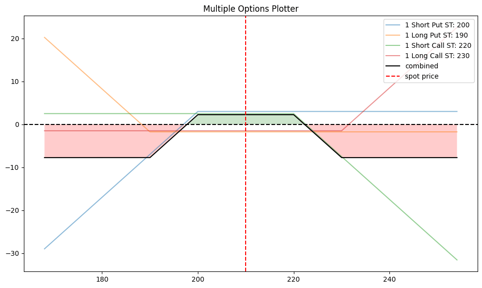
The payoff diagram explains the strategy perfectly.
- Maximum Profit: The flat, elevated section between the short strikes ($200 and $220). This is the net premium received: ($3.00 + $2.50) – ($1.75 + $1.50) = $2.25 per share.
- Maximum Loss: The flat sections on the far left and right. This loss is also defined and capped.
- Your Goal: For the stock to expire anywhere within that max profit range.
Conclusion
In this article, we’ve gone from the simple fundamental building blocks to multi-leg structures. We’ve seen how a single option can represent a straightforward bullish or bearish bet. More importantly, we’ve learned how to combine these blocks to craft strategies that align perfectly with a specific market outlook.
The key takeaway is that every option strategy has a unique risk and reward profile. It allows you to understand exactly what you stand to gain or lose before you ever put a dollar at risk.
Now that we have a good understanding of these strategies at expiration, our next step will be to explore the dynamic forces that affect an option’s value during its life. In the next article, we will see how their prices react to changes in the underlying stock price, the passage of time, shifts in volatility, and interest rate fluctuations.
