In our first article, we mapped out the world of options at a single, critical moment in time: expiration. We learned to read payoff diagrams, which clearly define our potential profit or loss based on where the underlying stock price lands on final day. This is a vital skill, but it only tells half the story. The reality is that from the moment you buy or sell an option until the day it expires, its value is in constant flux.

An option’s price isn’t a static number; it’s a living, breathing value that responds to the ever-shifting tides of the market. What drives these changes? Four primary forces are at play:

• The Underlying Stock Price: The most obvious and powerful driver.
• Time to Expiration: An option is a contract with a deadline, and time is a crucial component of its value.
• Implied Volatility: The market’s collective forecast of how much the stock will swing.
• Interest Rates: A subtle but important factor related to the cost of money.

The sensitivities of an option’s price to these factors are famously known in the trading world as “the Greeks” (Delta, Gamma, Theta, Vega, and Rho). While their mathematical definitions involve calculus, we can develop an intuitive understanding by using Python to model and visualize their effects.

In this article, we will dissect each of these dependencies, transforming abstract concepts into concrete, visual insights. By the end, you’ll understand not just what an option is worth at expiration, but why its value changes every single day.

1. Dependency on Stock Price: The Power of Delta

The most direct relationship is between an option’s price and the price of its underlying stock. As the stock price moves, the probability of an option finishing “in-the-money” (ITM) changes, directly impacting its value.

• For a Call Option: As the stock price rises, the call becomes more valuable.
• For a Put Option: As the stock price rises, the put becomes less valuable.

This sensitivity is known as Delta. Delta measures how much an option’s price is expected to change for a $1 move in the underlying stock. It ranges from 0 to 1 for calls and -1 to 0 for puts.

Let’s use the option price library in Python to see this in action. We’ll model a European option with a strike price (K) of $100, 30 days to expiration, 20% volatility, and a 5% risk-free interest rate.

import numpy as np
import matplotlib.pyplot as plt
from scipy.stats import norm

# Black-Scholes formula for European options
def black_scholes(option_type, s0, k, t, sigma, r):
    """
    Calculates the price of a European call or put option.
    
    option_type: 'call' or 'put'
    s0: Initial stock price
    k: Strike price
    t: Time to expiration in years
    sigma: Volatility of the stock
    r: Risk-free interest rate
    """
    d1 = (np.log(s0 / k) + (r + 0.5 * sigma ** 2) * t) / (sigma * np.sqrt(t))
    d2 = d1 - sigma * np.sqrt(t)
    
    if option_type == 'call':
        price = s0 * norm.cdf(d1) - k * np.exp(-r * t) * norm.cdf(d2)
    elif option_type == 'put':
        price = k * np.exp(-r * t) * norm.cdf(-d2) - s0 * norm.cdf(-d1)
    else:
        raise ValueError("Invalid option type. Choose 'call' or 'put'.")
        
    return price

# Define a range of stock prices to analyze
stock_prices = np.arange(60, 150, 1)

# Initialize lists to store option prices
call_prices = []
put_prices = []

# Calculate option prices for each stock price
for price in stock_prices:
    call_price = black_scholes('call', s0=price, k=100, t=30/365.0, sigma=0.20, r=0.05)
    put_price = black_scholes('put', s0=price, k=100, t=30/365.0, sigma=0.20, r=0.05)
    call_prices.append(call_price)
    put_prices.append(put_price)

# Plot the results
plt.figure(figsize=(10, 6))
plt.plot(stock_prices, call_prices, label='Call Option Price')
plt.plot(stock_prices, put_prices, label='Put Option Price')
plt.xlabel('Stock Price ($)')
plt.ylabel('Option Price ($)')
plt.title('Option Price vs. Stock Price')
plt.axvline(x=100, color='r', linestyle='--', label='Strike Price (K=100)')
plt.grid(True)
plt.legend()
plt.show()

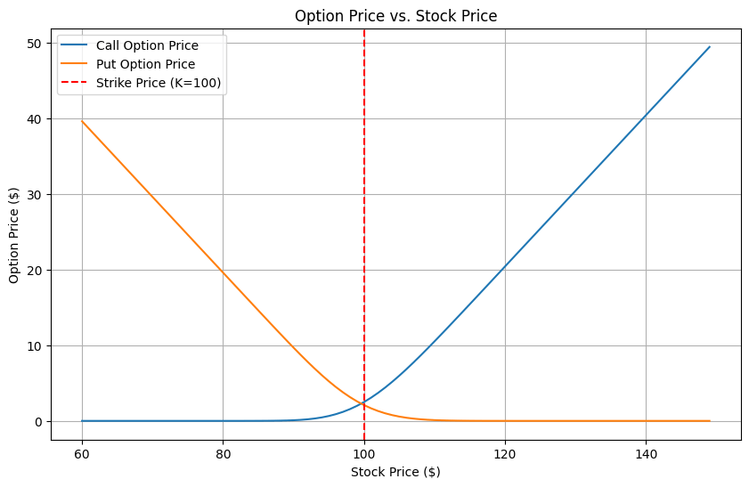
The chart elegantly illustrates the core concept:

1. The blue line (call option) slopes upward, showing its value increases with the stock price.
2. The orange line (put option) slopes downward, as its value erodes when the stock price climbs.
3. Notice the curves aren’t straight lines. The slope, the Delta, changes. For an option that is deep out-of-the-money (OTM), the line is nearly flat; its value is barely affected by a $1 stock move. For an option deep in-the-money (ITM), the line is steep, and the option’s price moves nearly one-for-one with the stock.

This change in Delta is itself a Greek, called Gamma, which measures the rate of change of Delta. Gamma is highest for at-the-money (ATM) options, meaning their sensitivity to stock price moves is the most dynamic.

2. Dependency on Time: The Inexorable Melt of Theta

An option’s value has two components: intrinsic value (how much it’s in-the-money) and extrinsic value (also known as time value). Extrinsic value is the premium you pay for the possibility that the option will become profitable by expiration. As time passes, that window of possibility shrinks, and so does the extrinsic value.

This decay in an option’s price due to the passage of time is called Theta. It is often referred to as the “time melt” or “time decay” of an option.

• Theta is the enemy of the option buyer and the friend of the option seller.
• The rate of decay is not linear. It accelerates as the expiration date approaches.

Let’s visualize this. We’ll fix the stock price at $100 (ATM) and plot the option’s value against the number of days remaining until expiration.

# Define a range of days to expiration
days_to_expiration = np.arange(1, 181, 1)

call_prices_time = []
put_prices_time = []

# Calculate option prices for each time to expiration
for days in days_to_expiration:
    # Convert days to years for the formula
    time_in_years = days / 365.0
    call_price = black_scholes('call', s0=100, k=100, t=time_in_years, sigma=0.20, r=0.05)
    put_price = black_scholes('put', s0=100, k=100, t=time_in_years, sigma=0.20, r=0.05)
    call_prices_time.append(call_price)
    put_prices_time.append(put_price)

# Plot the results
plt.figure(figsize=(10, 6))
plt.plot(days_to_expiration, call_prices_time, label='ATM Call Option Price')
plt.plot(days_to_expiration, put_prices_time, label='ATM Put Option Price')
plt.xlabel('Days to Expiration')
plt.ylabel('Option Price ($)')
plt.title('Option Price vs. Time to Expiration (Time Decay)')
plt.grid(True)
plt.legend()
plt.show()

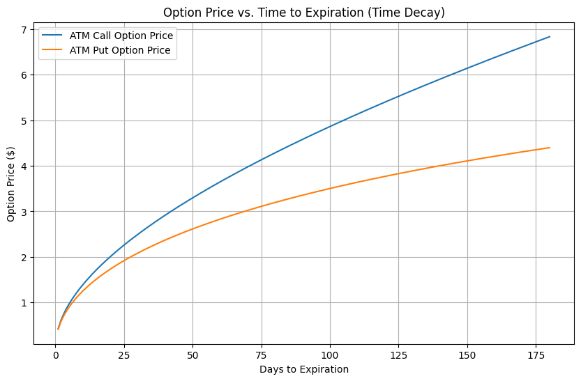
The graph reveals a crucial insight. The decay is slow and gradual when the option has many months of life left. But as it gets closer to expiration (the left side of the chart), the curve steepens dramatically. The value melts away at an accelerating rate, especially in the last 30-45 days. This is the Theta decay “waterfall,” a critical concept for all options traders.

3. Dependency on Volatility: The Fuel of Vega

What is volatility? In simple terms, it’s the magnitude of a stock’s price swings. Implied volatility is the market’s consensus forecast of how volatile the stock will be in the future. It’s a key ingredient in an option’s price because higher volatility means a greater chance of a large price move.

A large price move, in either direction, is good for the option buyer. A call buyer wants the stock to soar; a put buyer wants it to plummet. Higher volatility increases the probability of these extreme outcomes. Therefore, the higher the implied volatility, the more expensive an option becomes.

This sensitivity of an option’s price to a 1% change in implied volatility is called Vega.

• Vega is positive for both calls and puts.
• Option buyers are “long Vega” (they benefit from increasing volatility).
• Option sellers are “short Vega” (they benefit from decreasing volatility).

Let’s plot this relationship, keeping all other variables constant.

# Define a range of volatility values
volatilities = np.arange(0.05, 0.51, 0.01) # 5% to 50%

call_prices_vol = []
put_prices_vol = []

# Calculate option prices for each volatility level
for vol in volatilities:
    call_price = black_scholes('call', s0=100, k=100, t=30/365.0, sigma=vol, r=0.05)
    put_price = black_scholes('put', s0=100, k=100, t=30/365.0, sigma=vol, r=0.05)
    call_prices_vol.append(call_price)
    put_prices_vol.append(put_price)

# Plot the results
plt.figure(figsize=(10, 6))
plt.plot(volatilities, call_prices_vol, label='ATM Call Option Price')
plt.plot(volatilities, put_prices_vol, label='ATM Put Option Price')
plt.xlabel('Implied Volatility')
plt.ylabel('Option Price ($)')
plt.title('Option Price vs. Implied Volatility')
plt.grid(True)
plt.legend()
plt.show()

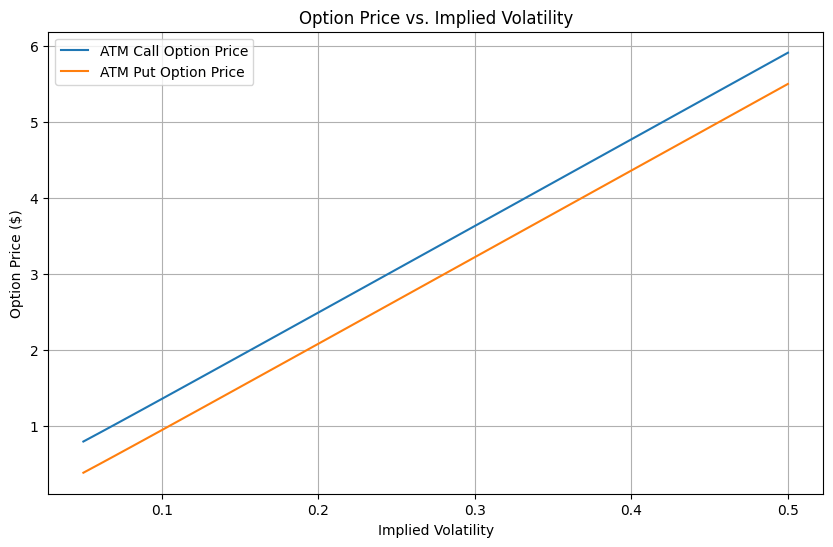
The result is clear and intuitive. As volatility (the x-axis) increases, the prices of both the call and the put option rise in tandem. This is why strategies like the Straddle and Strangle, which we discussed in the last article, are considered plays on volatility. You buy them when you expect volatility to increase, hoping the resulting price appreciation from Vega will outweigh the negative impact of Theta decay.

4. Dependency on Interest Rates: The Subtle Hand of Rho

The effect of interest rates is the least intuitive for most traders, but it’s rooted in the concept of present value and cost of carry. The sensitivity of an option’s price to a 1% change in the risk-free interest rate is known as Rho.

• Calls: Higher interest rates make call options more valuable. Why? Buying a call is a leveraged alternative to buying the stock outright. You pay a small premium to control 100 shares. The capital you saved by not buying the stock can be invested at the risk-free rate. The higher the rate, the more interest you earn, making the call a more attractive alternative.
• Puts: Higher interest rates make put options less valuable. A put gives you the right to sell stock and receive a fixed amount of cash (the strike price) in the future. Higher interest rates mean the present value of that future cash is lower, thus reducing the put’s value today.

# Define a range of interest rates
interest_rates = np.arange(0.01, 0.11, 0.01) # 1% to 10%

call_prices_rate = []
put_prices_rate = []

# Calculate option prices for each interest rate
for rate in interest_rates:
    call_price = black_scholes('call', s0=100, k=100, t=30/365.0, sigma=0.20, r=rate)
    put_price = black_scholes('put', s0=100, k=100, t=30/365.0, sigma=0.20, r=rate)
    call_prices_rate.append(call_price)
    put_prices_rate.append(put_price)

# Plot the results
plt.figure(figsize=(10, 6))
plt.plot(interest_rates, call_prices_rate, label='ATM Call Option Price')
plt.plot(interest_rates, put_prices_rate, label='ATM Put Option Price')
plt.xlabel('Risk-Free Interest Rate')
plt.ylabel('Option Price ($)')
plt.title('Option Price vs. Interest Rate')
plt.grid(True)
plt.legend()
plt.show()

Let’s model this final dependency.

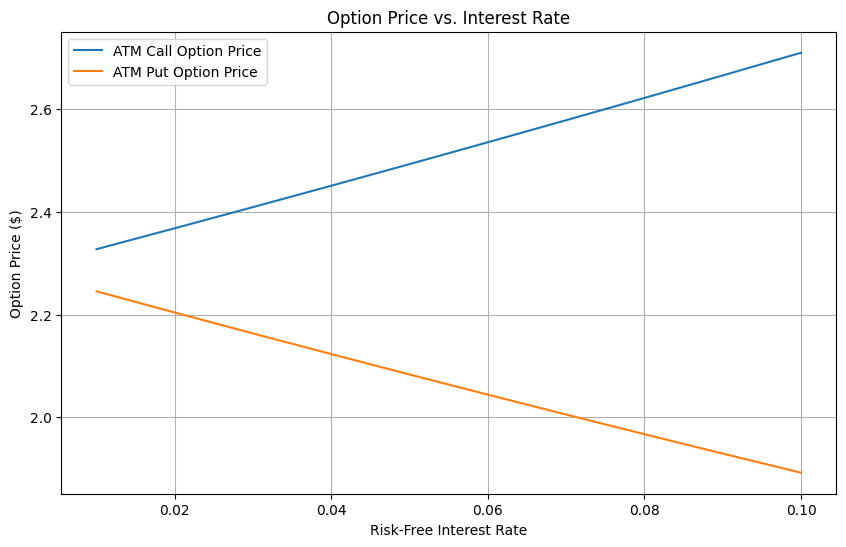
The chart confirms the theory: the call price inches up with rising rates, while the put price inches down. For short-term options, the impact of Rho is generally minimal compared to Delta, Theta, and Vega, but it is still a component of the pricing model.

Conclusion

We moved beyond the static world of expiration payoffs into the dynamic reality of its day-to-day life. We have seen, with the help of Python visualizations, that an option’s value is a sophisticated blend of four key ingredients: the underlying stock’s price (Delta), the relentless march of time (Theta), the market’s expectation of turbulence (Vega), and the cost of money (Rho).

Understanding these dependencies is what elevates a novice to an informed trader. It allows you to anticipate how your position will behave under different market conditions, to manage risk effectively, and to construct strategies. You no longer just see a price; you see the forces that shape it.

Now that we have a solid theoretical understanding of option payoffs and pricing dynamics, we are ready to step into the real world. In our next article, we will tackle the practical challenge of importing, cleaning, and analyzing actual options market data using Python.