

Beyond Price and Payoff: Why Options Require a Multi-Factor Risk Framework
Financial instruments like stocks have a straightforward, linear risk profile. Options, however, are fundamentally different. An option is a derivative contract, granting the holder the right, but not the obligation. This contractual nature creates a complex, non-linear relationship between the option’s value and the factors that influence it.
An option’s price is not only a function of the underlying asset’s price. Its value is an interplay of several variables: the price of the underlying, the time to expiry, the volatility of the underlying, and prevailing interest rates. As these factors fluctuate, the risk and reward profile of an options position changes, often in non-intuitive ways. A simple directional view is insufficient; traders must navigate a multidimensional risk landscape. To do this, they require a sophisticated set of tools to measure and manage these disparate risks.
Introducing the Greeks: A Dashboard for Navigating Option Risk
The “Greeks” are a set of measures that gives us a framework for understanding and quantifying the risks inherent in an options position. They act as a dashboard for the options trader, with each Greek serving as a gauge for a specific risk factor. These calculations allow traders to measure how different market conditions affect the price of an options contract. This enables them to make more informed decisions about buying, selling, and hedging.
The five primary Greeks, which form the foundation of options risk management, are:
- Delta (Δ): Measures the sensitivity of an option’s price to changes in the underlying asset’s price.
- Gamma (Γ): Measures the rate of change of Delta itself.
- Theta (Θ): Measures the sensitivity of an option’s price to the passage of time (time decay).
- Vega (ν): Measures the sensitivity of an option’s price to changes in volatility.
- Rho (ρ): Measures the sensitivity of an option’s price to changes in interest rates.
Mathematically, each Greek is a partial derivative of a pricing model. It isolates the impact of one variable while holding all others constant. This allows traders to decompose the total risk into its constituent parts, analyze each one, and manage them accordingly.
The Black-Scholes-Merton Model: The Engine of Calculation
The theoretical values for the Greeks are derived from a pricing model. The foundational model, which remains the industry standard for European-style options, is the Black-Scholes-Merton (BSM) model.
Core Assumptions and the “Perfect World” of BSM
The BSM model provides a theoretical value within a “perfect” financial market defined by a series of strict assumptions. Understanding these assumptions is critical to appreciating both the model’s power and its limitations:
- European-Style Options: The model is designed for options that can only be exercised at expiration.
- Lognormal Distribution of Prices: The model assumes that the price of the underlying asset follows a geometric Brownian motion, meaning that asset returns are normally distributed. This implies that asset prices themselves are log-normally distributed and cannot be negative.
- Constant Volatility and Risk-Free Rate: The model assumes that the volatility (σ) of the underlying asset and the risk-free interest rate (r) are known and constant throughout the option’s life.
- Frictionless Markets: There are no transaction costs or taxes, and all securities are perfectly divisible.
- No Dividends: The original Black-Scholes model assumed the underlying stock pays no dividends during the option’s life. The Merton extension adapts the model to account for a continuous dividend yield (q).
- No-Arbitrage: The model assumes there are no arbitrage opportunities.
The BSM Formulas for European Call and Put Options
Solving the Black-Scholes PDE under the appropriate boundary conditions yields the celebrated BSM formulas for the price of a European call and put option. The version presented here is the Merton extension, which incorporates a continuous dividend yield (q) and is more commonly used in practice.
The price of a call option is given by:

The price of a put option is given by:

Where the components are:
- S: Current price of the underlying asset
- K: Strike price of the option
- T−t: Time to expiration in years (τ)
- r: Continuously compounded risk-free interest rate
- q: Continuously compounded dividend yield
- σ: Volatility of the underlying asset’s returns
- N(⋅): The cumulative distribution function (CDF) of the standard normal distribution
- d1 and d2 are intermediate values calculated as:

Bridging Theory and Reality: The Pervasiveness and Pitfalls of BSM
Professional traders are acutely aware that the real world violates many of the BSM model’s core assumptions. Stock prices can experience sudden jumps, and volatility is not constant.
Given these known flaws, the persistence of the BSM model seem paradoxical. Its value on a modern trading desk lies not in its ability to perfectly predict prices. Instead, it serves as a standardized framework. It also acts as a common language. When a trader quotes an option’s “implied volatility” (IV), they are communicating the value of σ that must be plugged into the BSM formula to make the model’s price match the market price. This single number, IV, encapsulates the market’s collective opinion on the option’s “richness” or “cheapness”.
This transforms the BSM model from a flawed crystal ball into an indispensable ruler. Even if the ruler is slightly warped, it is the standard unit of measurement that everyone uses for comparison. As a result, the Greeks derived from this model become the standardized set of risk sensitivities.
A Deep Dive into the Primary Greeks
This part provides a detailed examination of each of the five primary Greeks. Each section will follow a consistent structure: a definition, the mathematical formula, a summary of key characteristics, a Python implementation , and an in-depth look at its practical application on a trading desk.
Delta (Δ) – The Compass of Directional Risk
Definition
Delta (Δ) is the first-order Greek and is arguably the most important because of its significant and immediate impact on an option’s value. It is defined as the first-order partial derivative of the option’s price (V) with respect to the price of the underlying asset (S).
Δ=∂V/∂S
In practical terms, Delta represents the expected change in an option’s premium for a $1 change in the price of the underlying, assuming all other factors remain constant.
Mathematical Formula (BSM)
Within the Black-Scholes-Merton framework, the formulas for Delta are as follows:
For a European Call Option:

For a European Put Option:

Key characteristics:
- Range: The Delta of a call option ranges from 0 to 1.0, while the Delta of a put option ranges from -1.0 to 0. A positive Delta indicates that the option’s price will increase as the underlying price rises, while a negative Delta indicates the option’s price will decrease.
- Moneyness: An at-the-money (ATM) option, where the strike price is equal to the underlying price, typically has a Delta close to +0.50 for a call and −0.50 for a put. As an option moves deep in-the-money (ITM), its Delta approaches ±1.0, meaning it behaves almost identically to the underlying asset. Conversely, as an option moves far out-of-the-money (OTM), its Delta approaches 0, making it less sensitive to price changes.
- Time to Expiration: As an option nears its expiration date, the behavior of Delta becomes more extreme. The Delta of an ITM option will accelerate towards ±1.0, while the Delta of an OTM option will accelerate towards 0. This is because with little time left, the probability of the option’s moneyness status changing diminishes.
Python Implementation
Calculating Delta in Python can be done from scratch using libraries like NumPy for mathematical operations and SciPy for the standard normal cumulative distribution function (norm.cdf). This approach is valuable for understanding the mechanics of the formula.
# Snippet: From-scratch Delta Calculation
import numpy as np
from scipy.stats import norm

def d1(S, K, T, r, q, sigma):
    """Calculates the d1 parameter for the Black-Scholes-Merton model."""
    if T <= 0 or sigma <= 0:
        return np.nan
    return (np.log(S / K) + (r - q + 0.5 * sigma**2) * T) / (sigma * np.sqrt(T))

def delta_call(S, K, T, r, q, sigma):
    """Calculates the Delta of a European call option."""
    d1_val = d1(S, K, T, r, q, sigma)
    if np.isnan(d1_val):
        return np.nan
    return np.exp(-q * T) * norm.cdf(d1_val)

def delta_put(S, K, T, r, q, sigma):
    """Calculates the Delta of a European put option."""
    d1_val = d1(S, K, T, r, q, sigma)
    if np.isnan(d1_val):
        return np.nan
    # Using the identity: N(d1) - 1 = -N(-d1)
    return np.exp(-q * T) * (norm.cdf(d1_val) - 1)

# --- Example Usage ---
S = 100      # Underlying price
K = 105      # Strike price
T = 0.5      # Time to expiration (6 months)
r = 0.05     # Risk-free rate (5%)
q = 0.02     # Dividend yield (2%)
sigma = 0.20 # Volatility (20%)

call_delta_val = delta_call(S, K, T, r, q, sigma)
put_delta_val = delta_put(S, K, T, r, q, sigma)

print(f"Call Delta: {call_delta_val:.4f}")
print(f"Put Delta: {put_delta_val:.4f}")
For professional applications, libraries such as py_vollib offer optimized and robust implementations.
Practical Trading Desk Application
On a trading desk, Delta is used in three primary ways that go far beyond its simple definition.
- Delta as a Hedge Ratio: This is the cornerstone of institutional options trading and risk management. The Delta of an option or a portfolio of options represents its equivalent exposure in the underlying asset. For example, a portfolio with a total Delta of +500 has the same directional risk as holding 500 shares of the underlying stock. To neutralize this directional risk, a process called delta hedging, a trader would sell 500 shares of the stock or an equivalent amount of futures contracts. This creates a “delta-neutral” position, which is theoretically immune to small changes in the underlying’s price. This allows traders to isolate and trade other factors, such as volatility or time decay.
- Delta as a Proxy for Probability: Traders frequently use Delta as a quick, back-of-the-envelope estimate for the probability of an option expiring in-the-money. A call option with a Delta of 0.30 is considered to have approximately a 30% chance of finishing ITM at expiration. For instance, traders selling OTM options to generate income will often target options with low deltas (e.g., 0.10 to 0.20) to increase their odds of the options expiring worthless.
- Delta as “Share-Equivalent” Exposure: At a portfolio level, the sum of all individual position deltas provides the desk’s total “delta-one” or share-equivalent exposure. A risk manager will monitor this aggregate Delta against strictly enforced limits. If a desk’s limit is ±50,000 share-equivalents of a particular stock, a total portfolio delta of +60,000 would represent a limit breach, requiring the head trader to reduce directional exposure immediately.
Gamma (Γ) – The Accelerator of Risk
Definition
Gamma (Γ) is a second-order Greek that measures the rate of change of an option’s Delta. It is formally defined as the second partial derivative of the option’s price (V) with respect to the underlying asset’s price (S), or equivalently, the first partial derivative of Delta with respect to S.

If Delta is analogous to the “speed” at which an option’s price changes, then Gamma is its “acceleration”. It quantifies how much an option’s Delta is expected to change for a $1 move in the underlying’s price.
Mathematical Formula (BSM)
In the BSM model, the formula for Gamma is the same for both call and put options:
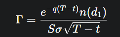
Where n(⋅) is the probability density function (PDF) of the standard normal distribution.
Key Characteristics
- Sign: Gamma is always positive for long options and always negative for short options. A positive Gamma means that as the underlying price moves in a favorable direction, the position’s Delta also becomes more favorable (i.e., profits accelerate). A negative Gamma means that as the underlying moves against the position, the Delta also becomes more adverse (i.e., losses accelerate).
- Moneyness and Time: Gamma is at its highest for options that are at-the-money. Its value diminishes for options that are deep ITM or far OTM. The most dramatic characteristic of Gamma is its behavior near expiration. For ATM options, Gamma increases exponentially as the expiration date approaches, a phenomenon often termed a “gamma explosion.” This makes the Delta of near-term ATM options extremely unstable.
Python Implementation
The Gamma calculation builds upon the d1 function defined previously.
# Snippet: From-scratch Gamma Calculation
def gamma(S, K, T, r, q, sigma):
    """Calculates the Gamma of a European option."""
    d1_val = d1(S, K, T, r, q, sigma)
    if np.isnan(d1_val) or S <= 0 or sigma <= 0 or T <= 0:
        return np.nan

    pdf_d1 = norm.pdf(d1_val)
    return (np.exp(-q * T) * pdf_d1) / (S * sigma * np.sqrt(T))

# --- Example Usage ---
gamma_val = gamma(S, K, T, r, q, sigma)
print(f"Gamma: {gamma_val:.4f}")
Practical Trading Desk Application
Gamma is a critical risk metric, particularly for market makers and traders managing dynamically hedged portfolios. It is often described as the risk that manages the risk (Delta).
- Managing Delta-Hedge Stability (Gamma Risk): A delta-neutral portfolio is only truly neutral for an infinitesimally small price change. Gamma tells the trader how quickly and by how much their delta hedge will decay as the market moves. A portfolio with a large negative Gamma exposure, typically from selling a large number of near-term ATM options (like a short straddle), is exceptionally risky. A modest move in the underlying can cause the portfolio’s Delta to change dramatically, forcing the trader to re-hedge at unfavorable prices and leading to accelerating, or “convex,” losses. This is often referred to as being “short convexity.”
- Gamma Hedging: A key distinction in hedging is that while Delta can be hedged using the linear underlying asset (stock or futures), Gamma cannot. The underlying asset has zero Gamma. Therefore, to alter a portfolio’s Gamma profile, a trader must trade other options. For example, a trader who is short a straddle (and thus short a large amount of Gamma) might buy a cheaper, further OTM strangle. This transaction creates an Iron Condor, which still has a negative Gamma profile, but the long options of the strangle reduce the overall magnitude of the negative Gamma, making the portfolio’s Delta more stable and the risk more manageable.
- Gamma Scalping: This advanced, market-neutral strategy is designed to profit from market volatility rather than direction. A trader establishes a long-Gamma, delta-neutral position (e.g., by buying an ATM straddle and shorting stock to neutralize the initial Delta). As the stock price moves up or down, the positive Gamma causes the position’s Delta to change. The trader then “scalps” by re-hedging—selling stock as the price rises and buying stock as it falls, systematically realizing small profits. The strategic goal is for the accumulated profits from this scalping activity to be greater than the cost of holding the long-gamma position, which is primarily its negative Theta (time decay).
Next part …
Theta (Θ) – The Unrelenting Cost of Time
Vega (ν) – The Barometer of Volatility
Rho (ρ) – The Echo of Interest Rates
Coming Soon!